An MLAB Example: Chemical Kinetics Modeling

Below we show an interesting example of MLAB modeling for dimer kinetics. Suppose we have two substances, A and B which bind to form a complex C, and the substance C, in turn, binds with itself to form a dimer D. We thus have:

A + B <--> C with association constant k1 and disassociation constant k2, and

C + C <--> D with association constant k3 and disassociation constant k4.

Suppose further we mix 2 mmoles of A and 3 mmoles of B and measure the concentration in mmoles of both C and D at ten equally-spaced times between 0 and 70 seconds. From this data we wish to estimate the association and dissociation constants k1, k2, k3, and k4. We may proceed in MLAB as follows.

First we read in the data consisting of values of C and D given at the common times 0:70!10. Although common times are used here, this is not required.

 * data = (0:70!10) &' read(ddata,10,2)
 * type data

    time    c        d
  1: 7    1.065    0.0058
  2: 14   1.383    0.2203
  3: 21   0.9793   0.4019
  4: 28   1.107    0.3638
  5: 35   0.7289   0.456 
  6: 42   0.7236   0.5014
  7: 49   0.4674   0.715 
  8: 56   0.6031   0.4723
  9: 63   0.6149   0.7219
 10: 70   0.3369   0.7294

 * cdata = data col 1:2
 * ddata = data col (1,3)

Now we define our kinetic model so that c(t) is the concentration of C in mmoles at time t and d(t) is the concentration of D in mmoles at time t.

 * fct c't(t)=k1*(a0-c-2*d)*(b0-c-2*d)-k2*c-2*d't(t)
 * fct d't(t)=k3*c*c-k4*d
 * initial c(0)=0
 * initial d(0)=0
 * a0=2;b0=3

Now we guess the values of k1, k2, k3, and k4. We may use the results of equilibrium studies, analyzed by MLAB, to know values for the ratios k1/k2 and k3/k4.

 * k1=.02;k2=.002; k3=.02;k4=.002
 * constraints q={k1>0, k2>0, k3>0, k4>0}

Now we may curve-fit the two ode-system-defined functions, c and d, to estimate k1, k2, k3, and k4.

 * fit(k1,k2,k3,k4), c to cdata, d to ddata, constraints q
 final parameter values
   value               error                 dependency   parameter
   0.06916895493       0.02023902877         0.5830898606   K1
   0.01003638127       0.01500173275         0.5933235047   K2
   0.01427015399       0.002713671566        0.7642104538   K3
  3.458442141e-20      0.003966026698        0.7396366489   K4
 4 iterations
 CONVERGED
 best weighted sum of squares = 2.184931e-01
 weighted root mean square error = 1.168581e-01
 weighted deviation fraction = 1.207618e-01
 lagrange multiplier[4] = -3.832523108

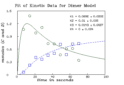
Now we may draw the results of the curve-fit.

 * m=integrate(c't,d't,0:100!140)
 * draw m col (1,2) color red
 * draw m col (1,4) color green lt dashed
 * draw cdata pt circle lt none color red
 * draw ddata pt circle lt none color green
 * bottom title "time in seconds"
 * left title "mmoles (C and D)"

 * view