A Numerical study of the Forced Damped Pendulum

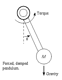
An ideal pendulum (i.e. with no friction) will swing back and forth (or loop in a full circle) forever if there is no outside force other than gravity acting upon it. Moreover, a pendulum with friction will come to rest if there is no other outside force besides gravity acting upon it. A more general forced damped pendulum with a periodic driving force pushing it shows more interesting asymptotic behavior than these two trivial cases. The angular position in radians as a function of time theta(t) of a forced damped pendulum is described by the following second order differential equation.

               theta''t + nu*theta't + sin(theta) = rho*sin(2*pi*f*t)
               theta(0) = theta0
               theta't(0) = s

where d^2*theta*dt^2 represents the inertia, nu*d(theta)/dt represents friction at the pivot, sin(theta) represents gravity, and rho*sin(2*pi*ft) represents a sinusoidal frequency f driving torque applied at the pivot. theta0 is the initial angular position and s is the initial angular velocity of the pendulum.

Numerical solutions show that both chaotic and periodic solutions of the forced damped pendulum equation are possible depending on the particular choice of system parameters nu, rho and f.

 "pendulum.do --- Solve the ODE for a forced pendulum"

 "the differential equation for the forced damped pendulum" 
 fct theta"t(t) = rho*sin(t) - c1*theta't - sin(theta) 
 "rho*sin(t) is the driving force, c1*theta't is friction, sin(theta) is gravity"

 "Read-in parameter values" 
 type "input the friction coefficient c1"; c1 = kread(); 
 type "input the driven force amplitude" rho = kread(); 
 type "input n: number of units of time to solve for"; n = kread();

 "Read-in the initial conditions" 
 type "Specify the initial conditions" 
 type "input theta(0)"; theta0 = kread(); initial theta(0) = theta0 
 type "input theta'(0)"; theta1 = kread(); initial theta't(0) = theta1

 "Specify the time values where we want the solution"
 data = 0:n:.1; "get an array from 0 to n at every .05"

 /* Now, integrate the differential equation. This is done implicitly 
 inside the operator 'points', the result matrix is put in the array m.
 The first column of m is the data array generated above, the second
 column is the theta value at the time corresponding to the time value in 
 the first column, the third column is the theta't value at the time 
 corresponding to the time value in the first column. */ 
 m = points(theta, theta't,data)

 "draw the trajectory (angular position vs. time)" 
 draw m col 1;2, color red 
 top title "Regular" 
 left title "Cumulative Angular Position"; 
 bottom title "Time" 
 view; "view the picture" 

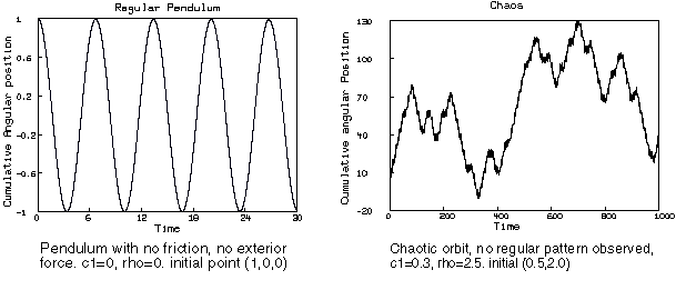
The following pictures are generated by this MLAB dofile. (with modified graphics). They are plots of time against the angular position. The left picture is the trivial regular case with a periodic orbit where c1 = 0 and rho = 0. The right picture shows a chaotic orbit where c1 = 0.3 and rho = 2.5. In all cases, the initial point corresponds to the initial conditions denoted by theta0 and theta1 in the dofile.

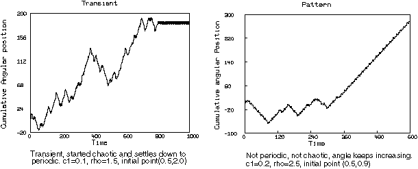
Here are another pair of pictures that are generated by the same dofile. The left picture shows a transient chaotic behavior which settles down to a periodic orbit after awhile. The parameter values are c1 = 0.1, rho = 1.5. The right picture shows another kind of behavior. It is not periodic, since the angle keeps increasing, it is not chaotic either since the the angle is increasing in a regular pattern, thus the Lyapunov exponent is not positive. The parameter values are c1 = 0.2, rho = 2.5.

To see a trajectory of a point in the phase-space (t, theta(t), theta'(t)) for the forced damped pendulum, we will construct an object called the Poincar'e map which is often used to reduce a continuous time system (or "flow") to a discrete time map with one less dimension. The basic idea of a Poincar'e map is to choose some appropriate hypersurface in the phase space and observe the intersection of the orbit in the phase-space with the surface. Since the solution of the system is unique with a given initial point, when we neglect numerical round-off error, each intersection point will uniquely determine the successive point. Thus, a continuous flow is reduced to a discrete map with one less dimension.

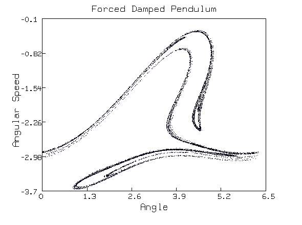
The picture above is the Poincar'e map of the trajectory of the point (0.5, 2.0) in the (theta(t), theta'(t)) reduced-dimension phase space for our forced damped pendulum system with the parameter rho = 2.5 and c1 = 0.3 which is the same as the chaos picture above. We used n = 10000. It is the Poincar'e return map with the section surface t = 0, which is equivalent to t = 2k*pi for any integer k since the variable t only appears in sin(t), and for any integer value of k, sin(2k*pi) will have the same value 0.

To compute the above Poincar'e map, we used almost the same MLAB dofile with only a few minor changes. We only want the solution at every time when t = 2k*pi (a multiple of 2*pi), Thus, we need to substitute the line for computing the time-list data in the above MLAB dofile with the following line:

  data = 0:(pi2*n):pi2; "get an array from 0 to pi2*n at every pi2"

 /* The variable theta is the angle of the arm of the pendulum. The angle 
 can range from 0 to pi2, any angle that is outside this region has a 
 corresponding angle in this region. We define a function to map all 
 the angles into 0:pi2 */ 
 fct ft(theta) = mod(theta, pi2) 
 m col 2 = ft on (m col 2); "map col 2 into the region 0 to pi2" 
 "draw a dot at each phase plane at each point (theta,theta't)" 
 draw m col 2:3, color red, lt none, pt dotpt 
 top title "Forced Damped Pendulum" 
 left title "Angular Velocity"; bottom title "Angle" 
 view; "view the picture" 

One can easily generate further pictures with other parameter values. More information about MLAB is available from:

Civilized Software Inc.
12109 Heritage Park Circle
Silver Spring, Md. 20906
Phone: (301)962-3711
FAX: (301)962-3712
Email: csi@civilized.com