Drug Combination Analysis in MLAB

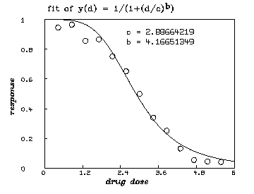
Suppose we have a set of drugs (or other treatments which we misclassify as ``drugs'' for the purpose of our analysis.) These drugs are supposed to be treatments for some disease, e.g. , HIV infection. Our goal is to assess whether, and to what extent, treatment with a particular combination of these drugs is more or less effective than some other such combination treatment. Such combination treatments include the case of treatment with a single drug, so we can also compare the efficacy of two distinct single drugs with our method.

For each treatment with a combination of drugs $D$₁,..., D _k , the data we have is a set of $k+1$ dimensional points of the form $(d$ ₁ ,...,d _k ,y) , where $d$ _j is the dose of drug $D$ _j (measured in any desirable units) and $y$ is the response observed in the subject represented by the point at hand.

The observed response is always non-negative, and is generally a value in the interval $[0,1]$. Such a value $y$ denotes the relative amount or level of disease present after the drug treatment. Thus a small response value indicates a better response than does a larger response value. Crudely, a response value $y$ should be measured such that $100(1-y)$ is the percent improvement observed. For example, let $w$ ₀ denote a subject's white blood cell count before treatment and let $w$ ₁ denote that subject's white blood cell count after treatment; then the response for that subject might be $1-(w$ ₁ -w ₀ )/w ₀ which is 1 minus the precentage improvement observed. The value 1 or greater denotes no suppression of disease, and values near 0 indicate substantial suppression of disease. Another example is that where we measure a quantity that is directly related to the level of disease present, such as the concentration of PSA present, normalized to lie in the interval $[0,1]$, although here, as in most cases, a percentage response is more appropriate, since the amount of disease present prior to treatment can vary greatly.

For a single drug, a so-called logistic dose-response curve often provides an adequate description of the effect of treatment with that drug. We assume that such a model for single drugs is appropriate here. (Although, see the remarks below on a non-parametric approach.) The general logistic dose-response function for a single drug is:

In our case, we assume that $a=1$ ( i.e. , we have no suppression of disease at 0 dose) and that $h=0$ ( i.e. , we approach complete suppression of disease as the dose becomes sufficiently large.) Thus, $y(d)=1/(1+(d/c)b)$. This dose-response curve generally ``decays'' sigmoidally from the value 1 to the value 0 as the dose $d$ increases. If $b>1$, we have faster decay, if , we have slower decay, if $b=0$, $y(d)$ is the constant value .5, and if , our dose-response curve inceases instead of decaying.

We may construct a single drug dose-response model for given dose-response data $(d$ ₁ ,v ₁ ),..., (d _m ,v _m ) by estimating the parameters $c$ and $b$ that fit the model function $y$ to our data via weighted least-squares minimization. An example showing the use of the MLAB mathematical and statistical modeling system[1] to read-in the dose-response data, define the single-drug logistic dose-response model function, provide initial guesses for the parameters $c$ and $b$, fit our model to the data to obtain the least-squares estimates of $c$ and $b$, and finally, to graph the results, is given below. (Often it is necessary to impose constraints on the parameters $c$ and $b$ in order to get a successful fit. This can be done in MLAB, but it is not needed in the example given here.)

* dv=read(d1data,100,2)
* fct y(d) = 1/(1+(d/c)^b)
* c = 3; b = 1

* fit (b,c), y to dv
final parameter values
      value               error                dependency    parameter
    4.166513485        0.3632194177         0.05378619542   B
    2.886642188       0.06692784189         0.05378619542   C
6 iterations
CONVERGED
best weighted sum of squares = 2.664797e-02
weighted root mean square error = 4.921934e-02
weighted deviation fraction = 5.824418e-02
R squared = 9.833524e-01

* draw points(y,0:6!100)
* draw dv lt none pt circle ptsize .02
* left title "response" font 18
* bottom title "drug dose" font 18
* top title "fit of y(d) = 1/(1+(d/c)'.5ub'.5d)" font 7
* title "c = "+c at (.5,.8)
* title "b = "+b at (.5,.75)
* view

Now let us consider a two-drug combination treatment. The dose-response model in this situation is a function of two arguments, $y(d$ ₁ ,d ₂ ) , that predicts the response to the combination dose $(d$ ₁ ,d ₂ ) . Let us suppose that drug $D$ ₁ and drug $D$ ₂ have no interaction. Moreover, we postulate that $y(d$ ₁ ,0)=1/ (1+(d ₁ /c ₁ )^b ₁ ) and $y(0,d$ ₂ )=1/(1+(d ₂ /c ₂ ) ^b ₂ ) . (The '^' symbol denotes the exponentiation operation; we must use it due to the inadequacies of HTML.) We assume that the parameters $c$ ₁ , $b$ ₁ , $c$ ₂ , and $b$ ₂ are known due to fitting the single-drug logistic dose-response model to given single-drug dose-response data for drug $D$ ₁ and separately for drug $D$ ₂ . In analogy to the terminology used with multivariate distribution functions, we may call the single-drug logistic functions $y(d$ ₁ ,0) and $y(0,d$ ₂ ) the marginal dose-response functions for the two-argument dose-response function $y$.

Let $h$ ₁ be the value such that our non-interaction two-drug dose-response model satisfies $y(\; h$ ₁ ,0)=r , and let $h$ ₂ be the value such that $y(0,\; h$ ₂ )=r . Now based on our no-interaction hypothesis, we can follow Bunow and Weinstein [2], and geometrically define $y(d$ ₁ ,d ₂ ) by postulating that $y(d$ ₁ ,d ₂ )=r for $(d$ ₁ ,d ₂ ) on the line-segment connecting $(\; h$ ₁ ,0) and $(0,\; h$ ₂ ) . Note it would not be appropriate to define $y(d$ ₁ ,d ₂ )= y(d ₁ ,0)+y(0,d ₂ ) since drug $D$ ₁ and drug $D$ ₂ compete to suppress the disease, even if they act independently; that is, when drug $D$ ₁ has acted to suppress some of the disease, there is less ``disease'' present for drug $D$ ₂ to apply to, and conversely. The line-segment connecting $(\; h$ ₁ ,0) and $(0,\; h$ ₂ ) is $L$ _r := (d ₁ ,d ₂ ) | (d ₁ ,d ₂ )= a ( h ₁ ,0)+(1- a )(0, h ₂ ), 0 < a < 1, and we specify that $y(d$ ₁ ,d ₂ )=r for $(d$ ₁ ,d ₂ ) belongs to the set $L$ _r . This is appropriate because, when drug $D$ ₂ is the same as drug $D$ ₁ , the predicted response to a combination dose $(d$ ₁ ,d ₂ ) must be the same as the predicted response to a dose of size $d$ ₁ +d ₂ of drug $D$ ₁ (or $D$ ₂ ) alone! Any drug-interaction model which fails to satisfy this condition cannot be a statistically-correct model.

Now note that, if $z=1/(1+(d/c)b)$, then $1=((1\; /\; z)-1)-1/b(d/c)$.

Recall that $y(\; h$ ₁ ,0)=r= 1/(1+( h ₁ /c ₁ )^[b ₁ ]) . Thus $1=((1\; /\; r)\; -1)^[-1/b$ ₁ ] ( h ₁ /c ₁ ) , so $a\; =((1\; /\; r)\; -1)^[-1/b$ ₁ ] ( a h ₁ /c ₁ ) . Also $y(0,\; h$ ₂ )=r= 1/(1+( h ₂ /c ₂ )^[b ₂ ]) , so $1=((1\; /\; r)\; -1)^[-1/b$ ₂ ] ( h ₂ /c ₂ ) , and thus $1-\; a\; =((1\; /\; r)\; -1)^[-1/b$ ₂ ] ((1- a ) h ₂ /c ₂ ) .

But then, when $(d$ ₁ ,d ₂ ) belongs to the set $L$ _r , $d$ ₁ = a h ₁ and $d$ ₂ =(1- a ) h ₂ for some value $a$ such that $0$< a < 1] , and we have specified that $y(d$ ₁ ,d ₂ )=r . Next, note that

This Bunow-Weinstein two-argument dose-response function for non-interacting drugs is a logically-correct generalization of a single-drug logistic dose-response function. This implicit function can be defined in MLAB as shown below. Note the care that is taken to avoid division by zero and raising zero to a negative power.

function y1(d1)=1/(1+(d1/c1)^b1)
function y2(d2)=1/(1+(d2/c2)^b2)

function y(d1,d2)=if d1=0 then y2(d2) else 
                  if d2=0 then y1(d1) else 
                  if y1(d1)<.00001 and y2(d2)<.00001 then 0 else 
                  if y1(d1)>.99990 and y2(d2)>.99990 then 1 else   
         root(z,1e-11,1-1e-11,(d1/c1)*(1/z-1)^(-1/b1)+(d2/c2)*(1/z-1)^(-1/b2) -1)

The MLAB commands used to produce a picture of the ``response-surface'' defined by our model function $y$ for two non-interacting drugs with identical marginal curves defined by $c$ ₁ =c ₂ =4.1665 and $b$ ₁ =b ₂ =2.8866 are given below. We assume the commands defining the functions $y$ ₁ , $y$ ₂ , and $y$ have been executed.

/* define c1=c2=2.8866 and b1=b2=4.1665 */
c1=2.8866; c2=c1; b1=4.1665; b2=b1

/* draw a 3D perspective view of the non-interaction drug response
   surface for two drugs having the same marginal single drug 
   dose-response curves. */
s = cross(0:6!20,0:6!20)
s col 3 = y on s

draw s linetype net
cmd3d("axes")
view 

The produced picture is shown below.

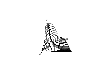
We may continue the above MLAB dialog to produce a contour map corresponding to the function $y$ with $c$ ₁ =c ₂ =4.1665 and $b$ ₁ =b ₂ =2.8866 corresponding to the surface shown above. The contour map shows some level lines where $y(d$ ₁ ,d ₂ ) is constant.

delete w3
/* draw a contour map corresponding to the surface above. */
draw contour(s) linetype vmarker
left title "drug-1 dose"
bottom title "drug-2 dose"
top title "c1=c2="+c+"  b1=b2="+b
view

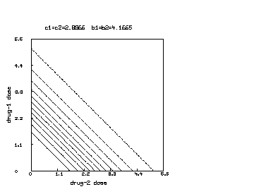
We may further continue the above MLAB dialog to produce a contour map corresponding to the function $y$ in the case where $c$ ₁ =2.08325 , $c$ ₂ =4.1665 and $b$ ₁ =b ₂ =2.8866 .

delete w
/* draw a contour map of the non-interaction combination drug 
   response surface where c1 is reduced to half of c2. */
c1 = c1*.5

s = cross(0:6!20,0:6!20)
s col 3 = y on s
draw contour(s) linetype vmarker
left title "drug 1 dose"
bottom title "drug 2 dose"
top title "c1="+c1+" c2="+c2+" b1=b2="+b1
view

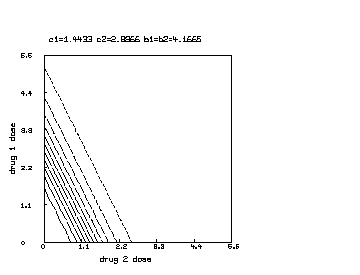
Finally, we may further continue the above MLAB dialog to produce a contour map corresponding to the function $y$ in the case where $c$ ₁ =c ₂ =4.1665 , $b$ ₁ =1.4433 and $b$ ₂ =2.8866 .

 
delete w
/* draw a contour map of the non-interaction combination drug 
   response surface where b1 is reduced to half of b2. */
c1 = c2; b1 = b1*.5

s col 3 = y on s col 1:2
draw contour(s) linetype vmarker
left title "drug 1 dose"
bottom title "drug 2 dose"
top title "c1=c2="+c+" b1="+b1+" b2="+b2
view

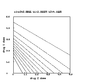
Note that the Bunow-Weinstein non-interacting two-drug dose-response function can be immediately generalized to the case of $k$ non-interacting drugs. In general we have:

Now we may consider drug combination treatments where the drugs involved may interact synergistically or antagonistically. To analyze such treatments, we need to have estimated the parameters $c$ ₁ , $b$ ₁ , $...$, $c$ _k , $b$ _k appearing in the marginal single-drug dose-response functions for the $k$ drugs under consideration, so that the Bunow-Weinstein non-interaction model is specified.

Given the data $(d$ _i1 ,d _i2 ,..., d_ik,v _i ) for $i=1,...,m$, we may compute the predicted non-interaction response values $r$ _i =y(d _i1 , d _i2 ,..., d_ik) . If we have no interaction, each $r$ _i value should be approximately the same as the corresponding observed response value $v$ _i . If not, then we can conclude there is evidence for a synergistic or antagonistic effect, and the size and direction of this effect can be estimated from the response differences $v$ _i -r _i . (Note that for the same combination of drugs, we might have both synergistic effects for dose-pairs in some regions and antagonistic effects in different dose-pair regions.)

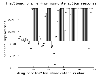
It may be convenient to consider the fractional differences $p$ _i :=1-v _i /r _i ; $100p$ _i is the percent change from the non-interaction predicted response $r$ _i that is observed in the actual response $v$ _i . If $v$ _i i , the disease was suppressed more than the non-interaction model would predict and $p$ _i >0 . If $v$ _i >r _i , the disease was suppressed less than the non-interaction model would predict and $p$ _i <0 . Crudely, we might say that our drug-combination exhibits a $100(p$ ₁ +...+p _m )/m percent mean synergy interaction effect.

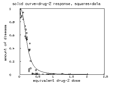
It is interesting to plot the $p$ _i -values, the $v$ _i -values and/or the $r$ _i -values versus the associated equivalent single-drug-dose of drug $D$ ₁ (or any other of the drugs involved) as determined by the Bunow-Weinstein non-interaction model $y$. If $(d$ ₁ ,...,d _k ) is the vector of dose values corresponding to the data-value $v$ _i and the predicted non-interaction value $r$ _i , then the equivalent drug $D$ ₁ dose is the value $e$ such that $y(e,0,...,0)=r$ _i . An MLAB function involving the root-operator can be defined to compute such equivalent dose values, but $e$ can be directly computed as $c$ ₁ / ((1 / r _i )-1)^[-1/b ₁ ] (with due care for $r$ _i =0 and for $r$ _i =1 .) Such plots may be useful in seeing how the synergy effect varies with dose.

Now one way to decide if the $r$ _i -values are, over all, sufficiently greater than the $v$ _i values to conclude that we have statistically-significant synergy is to test the hypothesis that the mean of the $p$ _i -values is less than or equal to 0 versus the alternate hypothesis that the mean of the $p$ _i -values is greater than 0. A similar test can be used to assess whether we have statistically-significant antagonism.

It is probably most appropriate to use a non-parametric test such as the Wilcoxon 2-sample paired-data test in MLAB on the $r$ _i -values versus the $v$ _i -values. And we can check our outcome with a paired-data $t$-test on the $p$ _i -values, even though the normal-distribution assumption used there may be invalid.

Note that in order to decide which of two drug combination treatments is better we need only compare the $p$ _i -values for treatment 1 with the $p$ _i -values for treatment 2.

Let us look at an example using MLAB to perform an analysis of some two drug combination responses at various doses. We have a file called ``a3azt.in'' which contains $n$ lines of three numbers, where the first number is the administered dose of drug $D$ <sub>1</sub> , the second number is the administered dose of drug $D$ <sub>2</sub> ,and the third number is the response measured as the amount of disease present after treatment (in this case, the response is the amount of virus assayed.) Each line in our data file is thus an ``observation'' from a single ``experiment''.

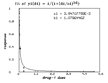
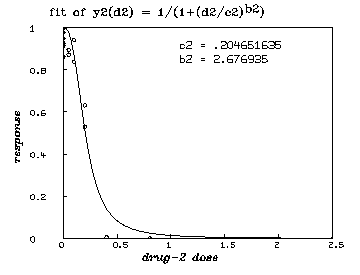
The MLAB dialog given below shows how we read our data, normalize the response values $v$ ₁ ,...,v _n to lie in $[0,1]$, extract the data for the marginal dose-response curves (one data-set where the drug $D$ ₁ dose is 0 and one data-set where the drug $D$ ₂ dose is 0), fit to obtain the estimated marginal dose-response curve parameters $c$ ₁ , $b$ ₁ , $c$ ₂ , and $b$ ₂ (which then define our Bunow-Weinstein non-interaction two-drug dose-response function), compute the predicted non-interaction response values $r$ ₁ ,..., r _n , and then compare the predicted $r$ _i -values with the observed $v$ _i -values to study the nature and amount of synergism apparent between our two drugs.

  
 /* read-in a3azt.in, normalize it, and extract the data needed to 
    fit the marginals. */
 m = read("a3azt.in",1000,3)
 m col 3 = (m col 3)/maxv(m col 3)
 m1 = extract(m,2,0) col (1,3); m1 = sort(m1)
 m2 = extract(m,1,0) col (2,3); m2 = sort(m2)

 /* define the non-interacting 2-drug combination model and its marginals */
 fct y1(d1) = 1/(1+(d1/c1)^b1)
 fct y2(d2) = 1/(1+(d2/c2)^b2)

 fct y(d1,d2) = if d1=0 then y2(d2) else 
  if d2=0 then y1(d1) else 
  if y1(d1)<.00001 and y2(d2)<.00001 then 0 else 
  if y1(d1)>.9999 and y2(d2)>.9999 then 1 else
  root(z,1e-11,1-1e-11,(d1/c1)*(1/z-1)^(-1/b1)+(d2/c2)*(1/z-1)^(-1/b2)-1)

 /* fit the marginals. the derivative y1'b1 involves the log
    of d1/c1 which may be 0.  Also the derivative y1'c1 involves
   (d1/c1)^(b1-1) which may become 0^0.  y2 has similar problems.
    To avoid these problems we can use symdsw = 0. */
 symdsw = 0
 constraints q = {b1 > .00001,b2 > .00001,c1 > .00001,c2 > .00001}
 c1 = 1; b1 = 1
 fit (c1,b1), y1 to m1 with weight ewt(m1), constraints q

final parameter values
      value               error                dependency    parameter
    0.039470779        0.0063108802         0.05395208237   C1
    1.078644618        0.2041472332         0.05395208237   B1
9 iterations
CONVERGED
best weighted sum of squares = 1.028776e+01
weighted root mean square error = 8.572280e-01
weighted deviation fraction = 7.954586e-02
R squared = 9.770071e-01
no active constraints

 c2 = 1; b2 = 2
 fit (c2,b2), y2 to m2 with weight ewt(m2), constraints q
 final parameter values
 
     value               error                dependency    parameter
    0.204651635        0.0231668295         0.07182693961   C2
    2.676935005        0.6159096057         0.07182693961   B2
11 iterations
CONVERGED
best weighted sum of squares = 4.343704e+01
weighted root mean square error = 1.647669e+00
weighted deviation fraction = 7.585580e-02
R squared = 9.646190e-01
no active constraints

 /* graph the resulting y1-fit. */
 draw points(y1,minv(m1 col 1):maxv(m1 col 1)!100)
 draw m1 lt none pt circle ptsize .01
 left title "response" font 18
 bottom title "drug-1 dose" font 18
 top title "fit of y1(d1) = 1/(1+(d1/c1)'.5ub1'.5d)" font 7
  title "c1 = "+c1 at (.5,.8)
 title "b1 = "+b1 at (.5,.75)
 view

 delete w

 /* graph the resulting y2-fit. */
 draw points(y2,minv(m2 col 1):maxv(m2 col 1)!100)
 draw m2 lt none pt circle ptsize .01
 left title "response" font 18
 bottom title "drug-2 dose" font 18
 top title "fit of y2(d2) = 1/(1+(d2/c2)'.5ub2'.5d)" font 7
 title "c2 = "+c2 at (.5,.8)
 title "b2 = "+b2 at (.5,.75)
 view

 delete w

 /* Now to analyze our drug combination data, we compute our non-interaction 
    response values r, and compare them to the actual data v.  If the v's 
    are smaller, we have synergism. Also we will look at the percent 
    changed-response values p.*/
 r = y on (m col 1:2)
 v = m col 3
 p = 1-v/'r

 /* Type out the average percentage-improvement seen in our
    data compared to the predicted non-interaction response. */
 type mean(p)
    = .593531217

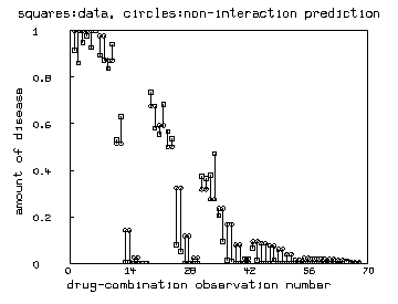
 /* Graph the linked-pairs of predicted noninteraction response and
    observed response for each drug-dose pair used. */
 draw v pt square lt none ptsize .01
 draw r pt circle lt none ptsize .01
 top title "squares:data, circles:non-interaction prediction"
 left title "amount of disease"
 bottom title "drug-combination observation number"
 n = nrows(v)
 nm = 1:n
 fct f(x) = if x < 0 then -1 else 1
 c = f on (v-r)
 qv = nm&'v&'c; qr = nm&'r&'c
 qq = mesh(qv,qr)
 qv = extract(qq,3,-1) col 1:2
 qr = extract(qq,3,1) col 1:2
 draw qv lt alternate color green
 draw qr lt alternate color red
 view

 
 delete w

 /* Graph the percentage-improvements (positive or negative) seen
    in each observation. */
 draw mesh(nm&'0, nm&'p) lt alternate color yellow
 draw p pt circle ptsize .01 lt none
 draw nm&'0 color red
 top title "fractional change from non-interaction response"
 bottom title "drug-combination observation number"
 left title "percent improvement"
 view

 delete w

 fct ed2(r) = if r=1 then 0 else if r=0 then maxd2 else c2/[(1/r-1)^(-1/b2)]
 maxd2 = maxv(m col 2)
 e = ed2 on r
 draw e&'v color green lt none pt square ptsize .01
 /* also show the drug-2 marginal curve */
 draw points(y2,minv(m2 col 1):maxv(m2 col 1)!100)
 top title "solid curve:drug-2 response, squares:data"
 bottom title "equivalent drug-2 dose"
 left title "amount of disease"
 view

 
 /* Now we use the Wilcoxon 2-sample test for paired data to compare our data
    v with the corresponding predicted non-interaction response values r. */
 wil2t(v,r)
[Wilcoxon 2 sample signed-rank test: are the medians of the
ranks of the observed paired data d1[] and d2[] plausibly equal?]
null hypothesis H0: median(d1) = median(d2).
The sum of positive ranks W-sample: T+ = 459.000000
The absolute sum of negative ranks W-sample: T- = 1819.000000

The probability P(W > 459.000000) = 0.999989
This means that a value of T+ at least as large as 459.000000 arises
about 99.998920 percent of the time, given H0.

The probability P(W > 1819.000000) = 0.000011
This means that a value of T- at least as large as 1819.000000 arises
about 0.001050 percent of the time, given H0.

The probability P[W > 1819.000000 or W < 459.000000] = 0.000022
This means that a rank-sum value at least as extreme as 1819.000000
arises about 0.002160 percent of the time, given H0.

: a  6 by 1 matrix TP

  1: 67           
  2: 459          
  3: 1819         
  4: .999989202   
  5: 1.05008711E-5
  6: 2.15957906E-5

In the wil2t output vector TP above, if the probability reported in TP[5] is small then we can reject the null hypothesis of equal responses, with probability TP[5] of being correct, and we can conclude that the alternate hypothesis: TP[4] is small, then we can conclude that $median(v)>median(r)$ (corresponding to antagonism), and if TP[6] is small, we can conclude that $median(v)$ does not equal $median(r)$.

Note that the graphs presented above can be constructed and have interest in the more-general situations of more than two drugs being used in combination.

When we have synergy, we will generally see that the bulk of the observed $v$ _i -values, plotted with respect to the equivalent dose $e$ _i of one of the drugs, lie below the marginal dose-response curve for that drug. This occurs above, where we compare the marginal curve for drug $D$ ₂ with our observed response vs. $D$ ₂ -equivalent dose amounts. We may fit a single-drug dose-response model to these $(e$ _i ,v _i ) points; the difference between this fitted curve and the single-drug marginal curve is a suitable basis for computing the degree of synergism or antagonism at that equivalent dose.

Sometimes we may have the situation where a drug $D$ ₂ has no theraputic effect, but may, nevertheless, modify the effect of another drug $D$ ₁ when used in combination. In this case, we should define the Bunow-Weinstein non-interaction model function so that $y(d$ ₁ ,d ₂ )= y(d ₁ ,0) ( i.e. , $y(d$ ₁ ,d ₂ )= 1/(1+(d ₁ /c ₁ )^[b ₁ ]) .) If this model does not fit our data, then we have statistically demonstrated the pure potentiation or inhibition behavior of drug $D$ ₂ on drug $D$ ₁ ,where drug $D$ ₂ , by itself, has no effect.

It is important to note that to use the approach to drug-combination analysis presented here, we must have the marginal single-drug dose-response curves specified by some means. If this is not possible, we can use a direct model-based approach due to Bunow and Weinstein. This approach requires that we fit an explicit model function to our drug combination data, where the model function contains explicit interaction terms. If the estimated interaction parameters are significantly different from their ``no-interaction'' value, then we have evidence for synergy or antagonism (but not both in different regions.)

One such drug-interaction model proposed by Bunow and Weinstein is:

In this model, the term $a$₁₂d ₂ ^[e₁₂] determines an change in the efficacy of drug $D$ ₁ in the presence of drug $D$ ₂ , which itself has an independent effect. When $a$₁₂ is 0, there is no interaction. The greater $a$₁₂ and $e$₁₂ are, the greater is the dose-dependent potentiation effect of drug $D$ ₂ on drug $D$ ₁ . When $a$₁₂ is negative, drug $D$ ₂ has an inhibitory effect on drug $D$ ₁ . Fitting such a model requires some care in the curve-fitting process. Numerical issues such as division by zero and zero raised to a negative power must be handled. Generally, appropriate weights are required, and often good initial parameter guesses and accompanying constraints are also needed. For example, it may be appropriate to constrain $e$₁₂ to be non-negative. MLAB can accept such weights and constraints, and with some care, can be used to estimate the desired parameters.

It is tempting to suppose that the estimated values of $C$ ₁ and $B$ ₁ determine the drug $D$ ₁ single-drug dose response curve, and likewise for $C$ ₂ and $B$ ₂ , but this is an unwarranted assumption. What we do know is that if $a$₁₂ is significantly different than 0 and $e$₁₂ is not a large negative value, then our data prefers to follow this interaction model, rather than the pure non-interaction model, and we take this as evidence of interaction. The basic underlying assumption is still that the actions of drug $D$ ₁ and drug $D$ ₂ separately are well-described by logistic dose-response curves as discussed above.

The entire drug-combination analysis method presented here can be recast in a more-general non-parametric framework. We can use a non-parametric estimate for each of our single-drug marginal dose-response curves, instead of using the logistic model. The Bunow-Weinstein non-interaction model can be defined with respect to these marginals, and the subsequent analysis proceeds as before. A suitable non-parametric estimate of a single-drug dose-response curve can be obtained in MLAB by first using the function MONOT to monotonize the data, and then using the function SMOOTHSPLINE to obtain an estimating optimal smoothing spline.

There is a serious practical problem with any drug-interaction analysis method which uses dose-response data as is done here. The problem is that at high (theraputic-level) doses, for some types of measurement of the amount of disease present, the error in the response-values may be so magnified that such measurements may be predominantly noise, and yet this is likely to be the domain in which treatment will actually occur. Practically speaking, it is much more important that there be no serious antagonism present than that our drug-combination be synergistic; as long as the drugs involved are not antagonistic and are jointly effective, it is generally useful to use them in combination. Of course such possible antagonism can be assayed via the analysis methods discussed here, subject to the same caveat of high errors in the response data. You might imagine that if synergism is seen at moderate ($IC$ ₅₀ -level) doses (where measurement error may be less problematical), then it will also be present at higher theraputic doses, but this is not always the case. The conclusion is that when the drugs involved can be usefully administered at levels where our observed responses will be predominately noise because of the nearly complete suppression of disease expected, drug-combination analysis does not take the place of clinical trials using the drugs at theraputic levels in order to assess the effacacy of the treatment.

[1] see www.civilized.com
[2] Bunow, Barry J. and Weinstein, John N. ''Combo: A New Approach to the Analysis of Drug Combinations in Vitro'', Annals N.Y. Acad. of Science Vol. 616, pp. 490-494, 1990.