This technical note shows the use of the MLAB mathematical and
statistical modeling system for solving the Hodgkin-Huxley differential
equations for arbitrary initial conditions.
The prevailing model of a nerve axon membrane is a pair of theories concerning the nature of the axon membrane with respect to active ("pumping'') and passive (diffusion) steady-state transport of various ions across the membrane and with respect to time-dependent "gate'' opening and closing which controls the active passage of ions through such "open gates''.
It is postulated that the membrane in a given state has a certain permeability for each given ion, and that this permeability is determined by the electrochemical potential across the membrane.
The permeability, PC, of a membrane for a particular chemical species, C, is a measure of the ease of diffusion of C across the membrane in the presence of a concentration difference on either side of the membrane. In particular, upon entering the membrane, one C-molecule will travel, on the average, (PCaF/(bRT))Em cm/sec transversely across the membrane, where PC = ubRT/(aF), and Em, u, b, R, T, a, and F are defined as follows.
For a given ionic species, C, which is placed in unequal concentrations on either side of an idealized membrane, there will be a diffusion of C in the direction of lower concentration. This diffusion changes any existing electric potential field, since charge is being redistributed. Other species may be diffusing as well, but regardless of the total complexity, the ionic current of C ions will be zero just when the electric potential difference across the membrane is sufficient to induce a compensating counter drift of C-ions in the direction of lower concentration. The potential difference of the potential in the "in''-compartment minus the potential difference in the "out''-compartment which leads to a net C-ion current of zero is given by the so-called Nernst potential difference, EC = ZRT/(ZF)log(Cout/Cin) volts, where Z is the valence of C (+1 for sodium and -1 for chlorine) and Cin and Cout are the concentrations of C in the inside and outside compartments. The actual electrical potential across the membrane is a function of the relative concentrations of each species present, and it is this total potential which determines how each ion would move with respect to its diffusion tendency. The total potential can be computed using the Goldman equation given below. Potential is defined so that positive charge flows towards points of lower potential, while negative charge flows towards points of higher potential. The membrane potential difference at a point is defined as the potential at the point minus the potential at a reference point in the outside solution.
For any given initial concentrations of various species and given time-course changes of membrane permeabilities for these species, there will be an associated change in total potential and a varying ionic current flow which, in principle, we can determine with appropriate equations. (We ignore the added complication of concentrations changing due to the diffusion of the solute, or of hydrostatic pressure gradients arising when solute diffusion is not possible.)
A full discussion of nerve membranes is given in ``Ionic channels of excitable membranes'' by Bertil Hille (Sinauer Associates, Sunderland, Mass, 1984).
For a giant squid nerve axon it has been experimentally determined that the chemical species of interest are potassium ions, sodium ions, chloride ions, and various other ions of lesser importance. Ions of all these less-significant species are collectively lumped together and called "leakage'' ions. Each of the various leakage ions have differing permeabilities; the result is that the permeability for leakage ions is an "average'' which compensates for the various differing permeabilities actually involved. Moreover, some of the leakage ions are negative and some are positive. We shall assume that our "average'' leakage ion is negative, and that the strength of an ionic current of leakage ions is diminished to compensate for this fiction. The resting axon membrane of an "average'' squid has permeabilities for these species which are given in the table below with the resting concentrations in mmoles/liter.
| inside | outside | resting permeability | potential difference | |
| K(+) | 400 | 10 | 6×10⁻⁶ | -72 mV |
| Na(+) | 50 | 460 | 8 ×10⁻⁹ | 55 mV |
| leakage(-) | 45 | 540 | -50 mV |
These values lead to a zero net ionic current in the resting state. The total
resting state potential difference, Er, based on the Goldman equation
works out to -60 mv. The Goldman equation in this
case is:
|
The above state cannot be indefinitely maintained by a passive membrane which allows each species to pass at a non-zero rate. Even though the net ionic current is zero, there are non-zero sodium, potassium, and leakage currents in the resting state. An additional mechanism is postulated, namely a "sodium pump'' which actively transports sodium ions from the inside to the outside to balance the resting state inward-diffusion, and a "potassium pump'' which transports potassium ions from the outside to the inside to balance the resting state outward-diffusion.
There is certainly such a mechanism present in the axon membrane but its precise chemical nature is not yet known. The energy to drive the pumps depends upon the conversion of ATP to ADP. It is not known how the two pumps are interrelated. It may be they are entirely independent, or they may be coupled in some way. There is probably not a single charge-balanced pump which brings one K ion inside for each sodium ion ejected outside, since the pump is required to compensate for unequal K and Na fluxes. A discussion of current research results about the pumping mechanism can be found in "The (Na++K+) activated enzyme system and its relationship to transport of Sodium and Potassium'' by Jens Chr. Skou, pp. 401:434 of Quarterly Reviews of Biophysics, Vol. 7, No. 3, July 1974.
Conductance is merely the reciprocal of resistance. It is a measure of the ability of a material to carry a particular ionic or electric current. Conductance is measured in W-1/cm2 units. The potassium conductance of one cm2 of axon membrane is denoted by gK, The sodium conductance of one cm2 of axon membrane is denoted by gNa, and the leakage ion conductance of one cm2 of axon membrane is denoted by gL. These values are, in general, functions of the potential difference history of the membrane.
Ohm's law holds for ionic current flow, but since there is zero current for the ionic species, C, when the voltage is exactly the Nernst potential, EC, for C, we have the C-ion current is given by IC = gC(Em-EC), where Em is the total membrane potential. Ohm's law applies here by convention, since gC is determined in any state, just so IC = gC(Em-EC) is true.
The conductance, gC, and the permeability, PC, for a
given ionic species, C, with charge Z, are related as follows.
|
The Hodgkin-Huxley model of an axon membrane is a mathematical description of the potential difference or voltage across the membrane which changes as a function of time in response to various perturbations of potential established with an associated applied current. It was presented in the Journal of Physiology, Vol. 117, pp. 500:544, 1952.
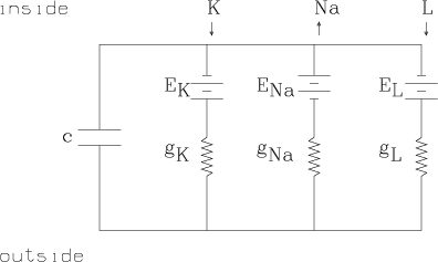
This description is in the form of an analogous circuit which in turn can be characterized by a set of non-linear differential equations. These equations contain an empirically adequate description of the feedback system which changes the conductances (or equivalently, the permeabilities) of the membrance as a function of time and potential difference.
The circuit merely contains the three main ionic current circuits in parallel together with the observed membrane capacitance.
Empirically we have the emf values EK » -72 mV, ENa » 55 mV, and EL » -50 mV.
The values gK, gNa, and gL are the conductances of the membrance for potassium, sodium, and leakage ions respectively. gK and gNa are functions of time and voltage.
The sign convention for current is such that a net flow of positive ions from inside to outside is a positive current. Thus a net flow of positive ions from outside to inside, or a net flow of negative ions from inside to outside is a negative current. Here current is measured in mAmperes per cm2, and Em, EK, ENa, and EL are measured in mvolts.
The values of EK, ENa, and EL given above imply that independently in the resting state, we would have a nearly-zero sodium current, a nearly-zero potassium current, and a zero leakage ion current. The sodium and potassium currents just balance the corresponding pump currents.
These circuits are connected in parallel however, and thus the total driving
potential applied to sodium ions is Em-ENa, the total driving potential applied to
potassium ions is Em-EK, and the
total driving potential applied to leakage ions is Em-EL. According to Kirchoff's law, the currents
into any point must sum to zero, so these three ionic currents must sum to 0.
From Ohm's law as discussed above, the sodium current, INa, is
gNa(Em-ENa), the
potassium current, IK, is gK(Em-EK), and the leakage ion current, IL,
is gL(Em-EL). But, in
the resting state, IK+INa+IL = 0, so
Em = (gNaENa + gKEK
+gLEL)/(gNa+gK+gL). In
the resting state, Em has been determined experimentally to be about
-60 mV, gNa has been determined to be
about .0106092 and gK is about .3666445, so we may define
|
(Usually, gL is set to .3, and EL is computed to yield a zero current, but we follow the opposite convention.)
Thus, for our ``average'' axon, the total sodium driving potential is -115 mV and we have a negative sodium current, the total potassium driving potential is 12 mV and we have a positive potassium current, and the total leakage ion driving potential is -10 mV and we have a negative leakage ion current.
The sodium current is approximately -1.22 mA, the potassium current is about 4.4 mA, and the leakage ion current is about -3.18 mA, and, of course, the sum is zero.
Of course, as these currents flow, the concentration-based emf's EK, ENa, and EL change; however the pumping devices postulated before are assumed to maintain a 1.22 mA sodium current and a -4.4 mA potassium current which forces leakage ions to remain in place in order to keep charge balanced in both the inside and the outside compartments. Thus in the resting state there is zero net ionic current across the membrane, and zero individual ionic currents as well. The Hodgkin-Huxley model does not include the pump current, so although there is zero net current in the resting state, the individual ionic currents are presented as computed above.
We may apply a time-varying current, Ia, across the membrane as a stimulus. This can be achieved by the feedback-controlled circuit shown below which applies whatever time-varying voltage, Va, across the membrane is needed to achieve the current Ia(t) at time t. Here time is measured in milliseconds.
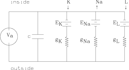
Thus, in general, we have Ia =
IK+INa+IL+Ic, where Ic is
the current across the membrane due to the capacitance c. Now Ic =
c(dEm/dt), where c » 1 mfarad/cm2. Thus, we obtain
|
The Hodgkin-Huxley model assumes that the emf's EK, ENa, and EL, and the conductance gL, are constant, but that the conductances gK and gNa are not constant, but rather are functions of the membrane potential difference history.
A change in gK corresponds to a change in the permeability of the membrane for potassium and similarly for gNa. The physical idea stated below underlying the Hodgkin-Huxley specification of how gK and gNa change is, by itself, incorrect, (see Armstrong, C., Physiological Reviews, Vol. 61, pp. 644:683, 1981). However, the associated equations adequately serve the purpose of defining gK and gNa as functions of time and membrane potential difference.
The Hodgkin-Huxley definition of gK and g Na can be "explained'' as follows.
Let the opening of a potassium ``channel'' which allows potassium to pass through the membrane involve j events. When j = 4, for example, we have (inside) K Û K¢Û K¢¢Û K¢¢¢Û K¢¢¢¢ (outside), and let us imagine that each such event is enabled by a K-gate molecule in the on-state. If n(t,E) is the proportion of K-gate molecules which are in the on-state at time t and membrane potential difference E, then nj is the probability that any given potassium channel is open; this probability is proportional to the probability that a potassium ion approaching the membrane will succeed in passing through. Note that j K-gate molecules might actually be one K-gate molecule which assumes 2j states, only one of which is "open''.
Suppose that when all the K-gate molecules are in the on-state, the associated potassium conductance of the membrane is [`g]K. In general, then, the potassium conductance of the membrane at voltage E and time t is [`g]Knj.
Suppose further, that K-gate molecules switch reversibly between the on-state and off-state following simple first-order kinetics; so that: dn/dt = f(an(1-n)- bnn), where f is a temperature compensating factor, and where the "rate constants'' an and bn are functions of voltage only! The factor f = 3(T-6.3)/10, where T is the temperature in degrees Celsius. Hodgkin and Huxley "guessed'' that an(E) = -.01(50+E)/(e-(50+E)/10-1) and bn(E) = .125e-(60+E)/80 by extensive numerical simulation and curve-fitting. The functions an and bn are chosen to "work''; their basic form was obtained from theoretical considerations, assuming that the potential across the membrane acts on charged particles (the gate molecules) to move them in and out of the way within the channels in the membrane.
For sodium, suppose there are both Na(1)-gate molecules and Na(2)-gate molecules, and let m(t,E) be the proportion of Na(1)-gate molecules in the on-state, and let h(t,E) be the proportion of Na(2)-gate molecules in the on-state, and finally, suppose opening a sodium channel across the membrane requires p Na(1)-events and q Na(2)-events. Thus, gNa = [`g]Namphq, where gNa is the sodium conductance when all the Na(1) and Na(2) gate molecules are in the on-state.
As before suppose that the Na(1) and Na(2) gate molecules are switching
between their on and off states following first order kinetics, so that dn/dt =
f(am(1-m)-bmm), and dh/dt = f(ah(1-h)-bhh), where again the
rate constants am, bm, ah, and
bh are functions of the potential
difference, E, which have been empirically chosen as:
| ||||||||||||||||||||
For a discussion of current knowledge and theory about the nature of the ionic channels, see "Ionic channels and gating currents in excitable membranes'' by Werner Ulbricht, pp. 7:31 in Annual Review of Biophysics and Bioengineering, Vol. 6, 1977, and "Kinetics of channel gating in excitable membranes'' by Leon Goldman, pp. 491:526 of Quarterly Reviews of Biophysics, Vol. 9, No. 4, Nov. 1976.
In general we may have an initial state where a "preconditioning'' ionic current, I0, has been applied for a time sufficient to establish a new steady-state. For any I0-value we have the resulting steady-state voltage, Ess, given by
Ess = rootE (IK+INa+IL-I0), where rootX(F(X)) denotes a value for X that makes F(X)=0.
Also, initially we assume n, m, and h are such that dn(0)/dt = dm(0)/dt = dh(0)/dt = 0, when an, bn, am, bm, ah, and bh are determined by the steady-state voltage, Ess.
Thus, we have: n(0) = nss(Ess), m(0) =
mss(Ess), and h(0) = hss(Ess) where,
| |||||||||||||||
|
The Hodgkin-Huxley model has j = 4, p = 3, and q = 1.
Note that it is possible to choose I0 so as to have Em(0) be any desired steady-state voltage, V, namely: I0 = rootI(Ess(I)-V). Such a choice for I0 represents a so-called voltage-clamp situation.
The stimulus current, Ia(t), is a current which varies as desired from the steady-state applied current I0. Ia(0) need not equal I0. The interpretation of this is that we have accomodated the axon membrane to the current I0, and then instantaneously switched the applied current to be Ia(0). Of course the variables, n, m, and h are accomodated to Ess(I0), not Ess(Ia(0)), so they will begin to change in response to this new voltage. Slightly more realism can be had by choosing Ia(t) = I0+(I1(t)-I0)(if t < s then (1-
Finally, it is possible to apply an impulse current which changes Em(0) by some desired amount, Vi, without allowing time for n(0), h(0) and m(0) to change. Thus our initial condition becomes Em(0) = Ess(I0)+Vi.
We have now given the complete Hodgkin-Huxley model for the giant squid axon membrane. There are various improvements; notably the Adelman-FitzHugh extension; however we shall suppose here that a ``naked'' axon having no Schwann cells is being modeled.
The following MLAB do-file, called HHF.DO, can be used to establish the Hodgkin-Huxley equations by typing DO HHF.
"file: HHF.DO";
EL=-50; ENA=55; EK=-72;
GKBAR=36; GNABAR=120; GL=.3179676;

FUNCTION PHI(TEMP)=3^((TEMP-6.3)/10);
FUNCTION F(X)=IF ABS(X)<.00002 THEN 1 ELSE X/(EXP(X)-1);
FUNCTION BM(E)=4*EXP((-E-60)/18);
FUNCTION BH(E)=1/(1+EXP(-3-.1*E));
FUNCTION BN(E)=EXP((-E-60)/80)/8;
FUNCTION AM(E)=F((-35-E)/10);
FUNCTION AH(E)=.07*EXP((-E-60)/20);
FUNCTION AN(E)=.1*F((-50-E)/10);
FUNCTION MINF(E)=AM(E)/(AM+BM(E));
FUNCTION HINF(E)=AH(E)/(AH+BH(E));
FUNCTION NINF(E)=AN(E)/(AN+BN(E));

K=25; S=.2;
FUNCTION IA(T)=I0+(I1-I0)*(IF T<S THEN 1-EXP(-K*T) ELSE \
   (1-EXP(-K*S))*EXP(-K*(T-S)));
FUNCTION IONIC(E,M,H,N)=GNABAR*M^3*H*(E-ENA)+GKBAR*N^4*(E-EK)+GL*(E-EL);
FUNCTION EM DIFF T(T)=IA(T)-IONIC(EM,M,H,N);
FUNCTION M DIFF T(T)=PHITEMP*(AM(EM)*(1-M)-BM(EM)*M);
FUNCTION H DIFF T(T)=PHITEMP*(AH(EM)*(1-H)-BH(EM)*H);
FUNCTION N DIFF T(T)=PHITEMP*(AN(EM)*(1-N)-BN(EM)*N);
FUNCTION ISS(E)=IONIC(E,MINF(E),HINF(E),NINF(E));
FUNCTION ESS(I)=ROOT(E,-246,830,ISS(E)-I);
"FOR ESS(I) LIES BETWEEN AND 830";

TEMP=6.3; PHITEMP=PHI(TEMP);
V0=-60; I0=0; ESS0=ESS(I0);
VI=0; I1=0;

INITIAL EM(0)=ESS0+VI;
INITIAL M(0)=MINF(ESS0);
INITIAL H(0)=HINF(ESS0);
INITIAL N(0)=NINF(ESS0);
The following MLAB do-file, called HHDO.DO, can be used to allow the user to establish any desired boundary conditions and then solve the Hodgkin-Huxley equations established with HHF.DO given above.
"file: HHDO.DO";
I0=0;
TYPE "
IF AN INITIAL VOLTAGE CLAMP OF X mV (-245<X%lt;-12) IS \
DESIRED, TYPE: V0=X.
OTHERWISE SET ANY DESIRED PRECONDITIONING uA CURRENT,Y, \
(-62<Y<1100) BY TYPING: I0=Y.
OTHERWISE TYPE A RETURN (V0 WILL BE -60 AND I0 WILL BE 0).";
DO KLINE;
IF V0 NOT=-60 THEN (I0=ISS(V0));
ESS0=ESS(I0);

VI=0;
TYPE "
ENTER INITIAL IMPULSE POTENTIAL CHANGE,X, BY TYPING: VI=X.
OTHERWISE TYPE A RETURN (VI WILL BE 0).";
DO KLINE;

I1=0;
TYPE "
DEFINE AN APPLIED CURRENT FUNCTION,IA, BY TYPING: \
FUNCTION IA(T)=desired expression. \
OTHERWISE, IF DESIRED, MERELY SET AN INITIAL .2 MSEC \
DURATION STEP CURRENT, s, (IN uA) BY TYPING: I1=s. \
OTHERWISE TYPE A RETURN (I1 WILL BE 0).";
DO KLINE;

TV=0:12:.1;
TYPE "
SET the TIME-VECTOR, TV, BY TYPING: TV=0:ft:dt (TV=0:12:.1 BY DEFAULT).";
DO KLINE;

METHOD = GEAR;
Q=INTEGRATE(EM DIFF T,M DIFF T,H DIFF T,N DIFF T,TV);
TYPE "
Q COL 1=TV, COL 2=EM, COL 3=EM', COL 4=M, COL 5=M', \
COL 6=H, COL 7=H', COL 8=N, COL 9=N'.";
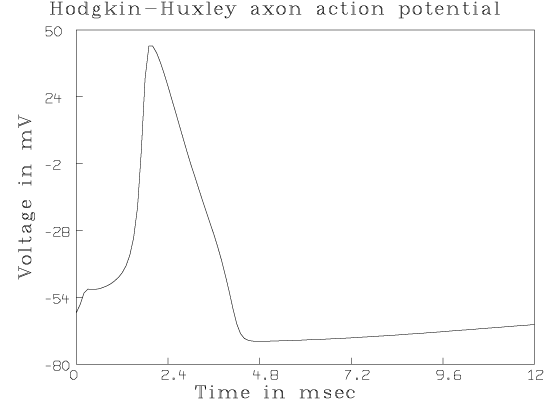
For example, we can compute the famous "action potential'' curve as follows.
*DO HHF
*DO HHDO

IF AN INITIAL VOLTAGE CLAMP OF X mV (-245<X<-12) IS DESIRED, TYPE: V0
= X. OTHERWISE SET ANY DESIRED PRECONDITIONING uA CURRENT,Y,
(-62<Y<1100) BY TYPING: I0 = Y. OTHERWISE TYPE A RETURN (V0 WILL BE
-60 AND I0 WILL BE 0).

*
ENTER INITIAL IMPULSE POTENTIAL CHANGE,X, BY TYPING: VI=X. OTHERWISE
TYPE A RETURN (VI WILL BE 0).
*

DEFINE AN APPLIED CURRENT FUNCTION,IA, BY TYPING: FUNCTION
IA(T)=desired expression. OTHERWISE, IF DESIRED, MERELY SET AN INITIAL
.2 SECOND DURATION STEP CURRENT,s, (IN uA) BY TYPING: I1 =
s. OTHERWISE TYPE A RETURN (I1 WILL BE 0).

*I1 = 50

SET the TIME-VECTOR, TV, BY TYPING: TV = 0:ft:dt (TV=0:12:.1 BY DEFAULT).

*

Q COL 1=TV,COL 2=EM,COL 3=EM',COL 4=M,COL 5=M',COL 6=H,COL 7=H',COL 8=N,COL 9=N'

*DRAW Q COL 1:2
*VIEW
The resulting picture with added titles is reproduced below.
Many familiar observations can be simulated and the model's response can be investigated by solving the Hodgkin-Huxley equations with various initial conditions. See "Computer analyses of the excitable membrane'' by T. Hironaka and S. Morimoto in Computers and Biomedical Research, Vol. 13, pp. 36:51, 1980, for a number of interesting numerical experiments which can be performed.
One problem with the Hodgkin-Huxley model is that current can flow in each loop of the circuit analog, but this implies sodium and potassium change into each other! This defect is not serious since the "impossible currents'' are small, but it is a conceptual error.
One of the main agreements of the Hodgkin-Huxley model with experiment is the suitability of the function Em(t) as a solution to the cable equation which involves the velocity of an action potential wave propagating along an axon.
Consider an infinitely-long sheathed cable of diameter d cm with ri W resistance for 1 cm. Let the exterior medium have a resistance of ro W for a 1 cm distance along the cable. Let Ie(x,t) be the current in mA applied to the surface of the short band of cable centered at the point at distance x along the cable and at time t with an electrode with a feedback voltage control which develops whatever voltage is required to obtain the specified current. The circuit is from ground through the electrode, then through the cable sheathing and, via leakage, back to ground. Let I(x,t) be the current in mA flowing across the short band of cable sheathing centered at position x, at time t. I(x,t) arises due to capacitance-driven current, leakage, and, for an axon, active forces in the membrane sheathing itself. Finally let V(x,t) be the voltage across the sheathing (inside potential minus outside potential) at position x and time t.
The cable equation relates these functions as:
|
For a constant sheathing resistance of Rm W per cm2, we have
|
If our cable is a giant squid axon, however, the membrane resistance varies,
and we may define I by the Hodgkin-Huxley equations as
|
Thus, we have
|
Another way to begin is to assume that Ie = 0, but that V(x,0) is
known as an initial condition, where the axon can be assumed to have been
charged by a current pulse function which established V(x,0) sufficiently
rapidly that m, h, and n have not responded. For example, we may have V(x,0) =
V0 ( exp)
(-x2/s2) for some spatial decay
constants. We have the additional constraint that V(x,t) ® -60 mV as t ® ¥, which will be necessarily satisfied.
The nature of the solution surface V for the initial condition V(x,0) =
V0 ( exp)
(-x2/s2) where V0 is above
threshold, is that the curve V(0,t) is an action potential-like curve which is
propagated along the axon (we ignore propagation towards x = - ¥) so that approximately the same
curve appears as V(x1, t+x1/q).
The parameter q is the propagation velocity. The initial part of the curve V(0,t) is artificially established by the initial condition and gradually dies out as time progresses, thus we do not have a pure traveling wave. The curve V(x1,t) for a large value of x1 is almost the same shape as V(x1+ e, t+(x1+ e)/q) however.
If we ignore the transient behavior and assume that t is translated so that
V(0,t) is propagated at velocity q cm/sec in a
nearly unchanged form, then we may take V(x,t) = V(x-
qt,0) = V(0,t-x/q). Let s = t-x/ q, and let U(s) = V(x,t) = V(0,t-x/q) = V(0,s). Then ¶2V/
¶x2 = (d2U/ds2)/ q2 and ¶V/ ¶t = dU/ds, and we have:
|
For U(0) = -60 mV and dU(0)/ds = 0, the solution is 0 but since V(x,t) ¹ -60 mV, even for t = 0 and very large x, when the surface V(x,t) is not flat at -60 mV, the appropriate initial conditions for the steady-state wave U is U(0) = U0 and dU(0)/ds = w0 where U0 and w0 are very small. m(0), h(0), and n(0) may revert to nearly the resting state values. To obtain a physically meaningful solution, the initial values U0 and w0 must be nearly correct. Also an acceptable solution must have U(s) ® -60 mV as s ® ±¥. This only occurs for certain discrete values of q. The parameter q is thus analogous to an eigenvalue of a linear operator.
It has been shown that, when U0, w0, and q are carefully chosen, then U(s) approximates the almost steady-state traveling wave observed in a real axon, and moreover that q is approximately the propagation velocity of about 168000/( pdc(ri+ro)) cm/sec which is actually observed. This fact constitutes one of the coroborations of the Hodgkin-Huxley model for the squid axon membrane.
Since q cannot be precisely represented, the numerically computed solution U(s) will not approach -60 mV as s® ±¥, but rather will approach + ¥ or -¥, depending upon the error in q (and U0 and w0).