Abstract: A powerful data analysis method based on the singular value decomposition is presented. An example of this method applied to data consisting of an absorption spectra surface is explained in detail. The MLAB mathematical modeling system is a suitable tool for doing a singular value decomposition analysis, and an example of this is presented.
Suppose we have a mixture of substances which we carry through a sequence of changes by varying some state variable. This process is called a titration with respect to the state variable, and the successive values of the state variable are called the titration levels. At each titration level, we measure some properties of the mixture; this data can then be modeled by a suitable mathematical description of the chemistry involved. When the measured properties are themselves a spectrum of responses to some sequence of stimuli, such as an absorption spectrum sampled over a range of wavelengths, a particularly elegant method of analysis called the "Singular-Value Decomposition'' (SVD) method due to Richard Shrager and Richard Hendler can be used [1]. The stimulus could even consist of the passage of time; thus kinetics data may be analyzed with this method. We will describe this method below in the context of an example with a titration with respect to hydrogen ion level, pH. (Hendler's actual experiments involved a titration with respect to electron content (i.e., voltage) corresponding to changes in the component substances of the respiratory chain in a mitochondrial membrane.)
For our example, suppose we have data values in a matrix A[1:m,1:n] such that Aik is the absorbance at wavelength wli of the mixture at titration pH-level pHk. We will take m = 70 and n = 27. The 70 wavelengths are equally spaced in the range from 350 nm to 650 nm. The 27 pH levels are equally-spaced in the range from pH 3 to pH 11.
We suppose there are t-1 substances in the mixture which appear in
greater concentration as the pH level is increased. The value t-1
is unknown and is to be estimated from the data. The relative
fraction of the jth substance is given by the Henderson-Hasselbalch
function:
|
Substance t and the other t-1 substances are each assumed to have a
characteristic absorption spectrum; gj(wl) denotes the absorbance
seen for 1 unit of substance j at wavelength wl. Often, but not
always, gj is approximately a gaussian bell-shaped curve centered
at a characteristic central wavelength. Absorption spectra are
assumed to be additive; the spectrum for several substances is the sum
of the spectra for each individual substance. Now we can compute the
overall absorbance bik at wavelength wli and pH-level pHk as:
|
Here, cj fj(pHk) is the concentration of substance j at pH-level pHk, and gj(wli) cj fj(pHk) is the absorbance at wavelength wli due to this concentration of substance j. When the pKj values appearing in the fj functions are correctly specified, bik should match the data value Aik.
We can express this model in matrix form as follows. Let F be an n×t matrix with Fkj = fj(pHk). Note that F col t = 1 identically. Let D be an m ×t matrix with Dij = gj(wli)cj. Note that D col t is the baseline spectrum at the m wavelengths being monitored. Let B be the m ×n matrix with Bik = bik. Then B = DFT, and B » A. (B would equal A exactly, except for measurement error.)
Given the data A, we wish to estimate t, and pK1,Ľ,pKt-1, and Dij for 1 Ł i Ł m and 1 Ł j Ł t, and Fkj for 1 Ł k Ł n and 1 Ł j Ł t. This may be done using the matrix singular-value decomposition. Note that if we know pK1,Ľ, pKt, we then know the elements of the matrix F, and conversely.
Any m × n real matrix A can be written as A = USVT, where U is an m × m orthogonal matrix, S is an m × n diagonal matrix with decreasing non-negative diagonal values called the singular values of A, and V is an n × n orthogonal matrix. The number of positive singular values exhibited in S is the rank of A.
In our example, we thus write A = USVT. Now we discard the zero or almost zero singular values from S, leaving t positive singular values in the modified t ×t diagonal matrix S. We have thus determined the value t; recall that the number of non-background substances is t-1. We also discard the last m-t columns of U and the last n-t columns of V that correspond to the discarded singular values to obtain U = U col 1:t and V = V col 1:t. We now have A » USVT. "Almost zero" can be defined as less than about 1% to 2% of the maximum singular value; however, this is a dangerous assumption. Shrager suggests we check the noise apparent in the corresponding columns of V; only singular values corresponding to significantly noisy columns of V should be discarded.
Now we may factor V as V = F H where H is a t ×t matrix, so
A = U S HT FT, and hence we may obtain D = U S HT, since A = DFT. In order to factor V into explicitly-known matrices F and H,
we use curve-fitting. Let:
|
Note that [qj(pH1),Ľ, qj(pHk)]T = V col j. Thus we may estimate H1j, H2j,Ľ,H(t-1)j, Htj, and pK1,Ľ,pKt-1 by fitting the model qj to the n × 2 data matrix Xj := (3:11!27) &'(V col j), for j = 1,Ľ,t. (Recall that in our example we are using 27 equally-spaced pH-values between 3 and 11.) This is best done by simultaneously fitting the function qj to the data points Xj using the constant weight value (Sjj )2 for 1 Ł j Ł t.
Now having estimated t, and pK1,Ľ,pKt-1, and the t2 elements of H, we may directly obtain the matrix F and then D.
The columns of D are the spectra of the t substances taken at their maximum concentrations; thus (D col j)T = cj[gj(wl1),Ľ,gj(wlm)]. If we know these spectral curves independently, we can deduce the concentration scale factors c1,Ľ,ct. Looking at these curves also serves as a check on the entire modeling process.
MLAB is an advanced mathematical and statistical modeling system, originally developed at the NIH, that is particularly suited for handling modeling and estimation problems in analytical chemistry. MLAB contains all the facilities needed to carry out the SVD analysis described above. Below is a particular MLAB dialog showing the SVD method applied for our example.
First we read in our data matrix A, where A is a 70 ×27 matrix whose rows correspond to the wavelengths 350:600!70 (nm), and whose columns correspond to the pH values 3:11!27. Aij is the absorbance observed at wavelength-level i and pH-level j.
*a = read(dataf,70,27)
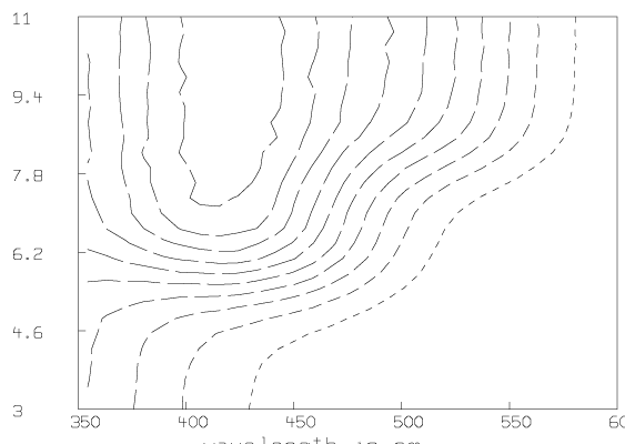
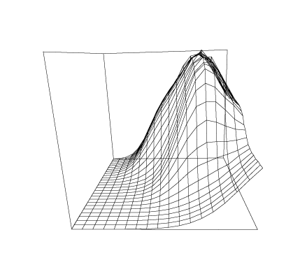
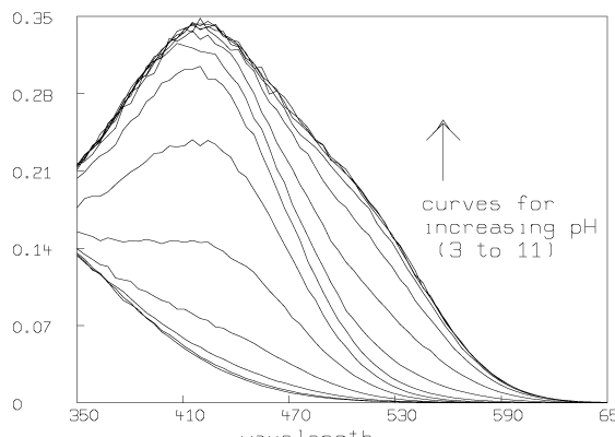
Some graphs which show the nature of the data A are given below. All of these graphs were drawn with MLAB.

Now we compute the singular value decomposition of A and decide the value of t.
* m=nrows(a); n=ncols(a)
*
* u=svd(a)
* s=(u row 1)'
* v=u row (m+2):(n+m+1)
* u = u row 2:(m+1)
* t=nrows(compress(((s col 1)>.025)&'s));
* type s row 1:(t+3); "type the singular values 3 beyond the t-th"

    : a  7 by 1 matrix

  1: 6.90549919
  2: .964371539
  3: .458168815
  4: 4.74121723E-2
  5: .023760869
  6: 2.21695634E-2
  7: .020740888

* v=v col 1:t; u= u col 1:t
*
* fct f1(ph)=1/(1+10^(pk1-ph))
* fct f2(ph)=1/(1+10^(pk2-ph))
* fct f3(ph)=1/(1+10^(pk3-ph))
* fct b1(ph)=h[t,1]+h[1,1]*f1(ph)+h[2,1]*f2(ph)+h[3,1]*f3(ph)
* fct b2(ph)=h[t,2]+h[1,2]*f1(ph)+h[2,2]*f2(ph)+h[3,2]*f3(ph)
* fct b3(ph)=h[t,3]+h[1,3]*f1(ph)+h[2,3]*f2(ph)+h[3,3]*f3(ph)
* fct b4(ph)=h[t,4]+h[1,4]*f1(ph)+h[2,4]*f2(ph)+h[3,4]*f3(ph)
*
* h=.3*shape(4,4,ran on 0^^16); "generate random guesses for h"
* pk1= 7; pk2 = 7.2; pk3= 6; "choose guesses for pk1,pk2,pk3"
*
* wl=350:650!70;
* phv=3:11!27
*
* maxiter=30; symdsw=0
* fit(h,pk1,pk2,pk3),b1 to phv&'(v col 1) with wt s[1]^^n,\
> b2 to phv&'(v col 2) with wt s[2]^^n,\
> b3 to phv&'(v col 3) with wt s[3]^^n,\
> b4 to phv&'(v col 4) with wt s[4]^^n
final parameter values
      value               error                dependency    parameter
 -0.04313096632      0.002075088787          0.8681882157   H[1]
  -0.5091112274      0.006380218701          0.9001594031   H[2]
  -0.4141844706      0.008460681648           0.880494897   H[3]
  -0.5124442081       0.02935544387          0.9040697608   H[4]
 -0.06083337034       0.01144532059          0.9974810125   H[5]
   0.2027353714       0.03290432573          0.9978176388   H[6]
  0.00747866897       0.07009215024          0.9989876919   H[7]
    2.848373276        0.4970101962          0.9998054387   H[8]
  -0.1143730484       0.01060867204          0.9973495801   H[9]
 -0.09979224416       0.03273355056           0.998006569   H[10]
   0.6236741131       0.06485462555          0.9989311313   H[11]
   -2.542220886        0.5055039097          0.9998299828   H[12]
 -0.04089842681      0.0009856221674          0.8092088134   H[13]
   0.2031173917      0.002508541316            0.78909474   H[14]
  -0.3226308862      0.003843686277          0.8109168102   H[15]
    0.152892387       0.01220313549          0.8187234648   H[16]
    8.006947711       0.01676401014           0.720544985   PK1
    6.058377382       0.05911112374          0.9828623017   PK2
    5.553356498       0.04694757727          0.9790372858   PK3
20 iterations
CONVERGED
best weighted sum of squares = 3.075587e-03
weighted root mean square error = 5.878534e-03
weighted deviation fraction = 3.081091e-03
R squared = 9.844744e-01
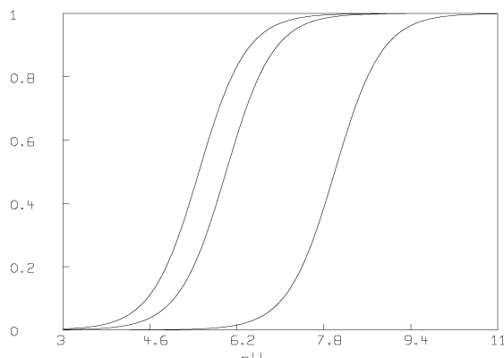
We have estimated t ( = 4) and pK1, pK2, and pK3 (pK1 = 8.007, pK2 = 6.058, pK3 = 5.553). We have also computed the matrix D. Now we present some pictures drawn in MLAB showing the results after this analysis of the data.
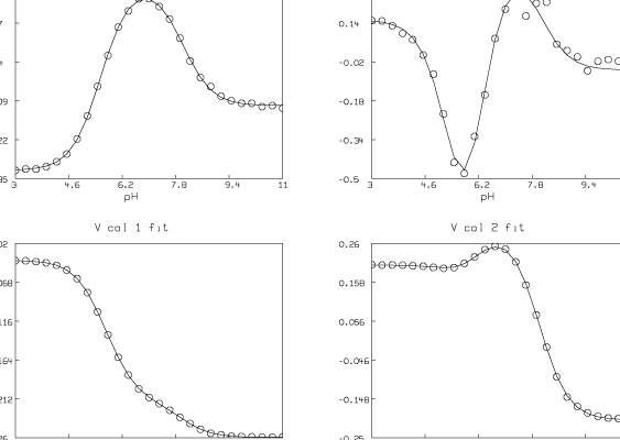
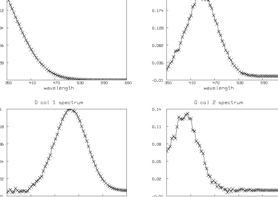
Although the fit we show here is very good, in general the fit we obtain can be very sensitive to the initial guesses for the parameters. Shrager and Hendler have developed a collection of heuristic techniques to acquire reasonable initial guesses. Also, the fact that the Hij parameters appear linearly means that a two-stage fitting approach consisting of separately fitting just the linear and then the nonlinear parameters could be used [2].
[1] Hendler R, Shrager R.; ``Analysis of the Spectra and Redox Properties of the Pure Cytochromes aa3'', Biophysical J. Vol. 49, pp. 717-729, March 1986.
[2] Golub and Peryra, ``Separable Least-Squares'', SIAM J. of Numerical Analysis, Vol. 10, No. 2, pp. 413:432, April 1973.