Solving Windkessel Models with MLAB
Windkessel models are frequently used to describe the load faced by the heart in
pumping blood through the pulmonary or systemic arterial system, and the
relation between blood pressure and blood flow in the aorta or the pulmonary
artery. Characterizing the pulmonary or systemic arterial load on the heart in
terms of the parameters that arise in Windkessel models, such as arterial
compliance and peripheral resistance, is important, for example, in quantifying
the effects of vasodilator or vasoconstrictor drugs. Also, a mathematical model
of the relationship between blood pressure and blood flow in the aorta and
pulmonary artery is useful, for example, in the development and operation of
mechanical heart and heart-lung machines. If blood is not supplied by these
devices within acceptable ranges of pressure and flow, the patient will not
survive.
This paper will briefly describe three Windkessel models and demonstrate the use of the MLAB mathematical modelling computer program in solving Windkessel model differential equations, estimating values of Windkessel model parameters from laboratory data, comparing differential equation models, and generating graphs that can be displayed on computer screens and incorporated into word processor documents. MLAB is the best commercially available software for these purposes.
A description of an early Windkessel model was given by the German physiologist Otto Frank in an article published in 1899 [6]. The model has been applied recently in studies of chick embryo [17] and rat [12]. It likens the heart and systemic arterial system to a closed hydraulic circuit comprised of a water pump connected to a chamber. The circuit is filled with water except for a pocket of air in the chamber. (Windkessel is the German word for air-chamber.) As water is pumped into the chamber, the water both compresses the air in the pocket and pushes water out of the chamber, back to the pump. The compressibility of the air in the pocket simulates the elasticity and extensibility of the major artery, as blood is pumped into it by the heart ventricle. This effect is commonly referred to as arterial compliance. The resistance water encounters while leaving the Windkessel and flowing back to the pump, simulates the resistance to flow encountered by the blood as it flows through the arterial tree from the major arteries, to minor arteries, to arterioles, and to capillaries, due to decreasing vessel diameter. This resistance to flow is commonly referred to as peripheral resistance.
Assuming the ratio of air pressure to air volume in the chamber is constant and the flow of fluid through the pipes connecting the air chamber to the pump follows Poiseuille's law and is proportional to the fluid pressure, the following differential equation is found to relate water flow and pressure:
|
(1) |
Here I(t) is the water flow out of the pump as a function of time measured in volume per time units, P(t) is the water pressure as a function of time measured in force per area units, C is the constant ratio of air pressure to air volume, and R is the flow-pressure proportionality constant.
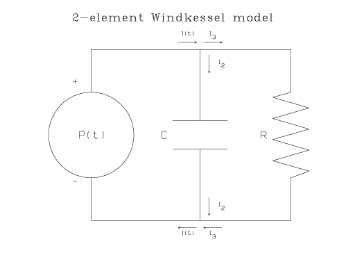
The same equation describes the relationship between the current, I(t), and the time-varying electical potential, P(t), in the following electrical circuit:
In this circuit, I2 is the current in the middle branch of the circuit, I3 is the current in the right branch of the circuit, R is the resistance of the resistor, and C is the capacitance of the capacitor. Because there are only two passive elements in this circuit, the resistor and capacitor, this model is commonly referred to as the 2-element Windkessel model.
According to Ohm's Law, the drop in electrical potential across the resistor is I3 R. The drop in electrical potential across the capacitor is Q/C, where Q is the instantaneous charge on the capacitor and [dQ/dt] = I2. From Kirchhof's First Law, the net change in electrical potential around each loop of the circuit is zero; therefore P(t) = I3 R and P(t) = Q/C. From Kirchhof's Second Law, the sum of currents into a junction equals the sum of currents out of the same junction: I(t) = I2+I3. Eliminating I2 and I3 from the junction equation leads to the the differential equation shown above.
In terms of the physiological system, I(t) is the flow of blood from the heart to the aorta (or pulmonary artery) measured in cubic centimeters per second (cm3/sec), P(t) is the blood pressure in the aorta (or pulmonary artery) in millimeters of mercury (mmHg), C is the arterial compliance in the aorta (or pulmonary artery) in units of cubic centimeters per millimeter of mercury (cm3/mmHg), and R is the peripheral resistance in the systemic (or pulmonary) arterial system in units of millimeters of mercury per cubic centimeter per second (mmHg.s/cm3).
During diastole, when there is no blood flow from the heart, I(t) = 0 and the Windkessel equation can be solved exactly for P(t):
|
(2) |
where td is the time at the start of diastole and P(td) is the blood pressure in the aorta (or pulmonary artery) at the start of diastole.
Another model of the circulatory system is the Broemser model, which was described by the Swiss physiologists Ph. Broemser and Otto F. Ranke in an article published in 1930 [3]. Also known as the 3-element Windkessel model, the Broemser model adds a resistive element to the 2-element Windkessel model between the pump and the air-chamber to simulate resistance to blood flow due to the aortic or pulmonary valve. More recently it has been used to study blood pressure and flow in the aorta of chick embryo [16,17], and dog [5], and in the pulmonary artery of pig [10].
Here is a schematic of the electrical circuit corresponding to the 3-element Windkessel model:
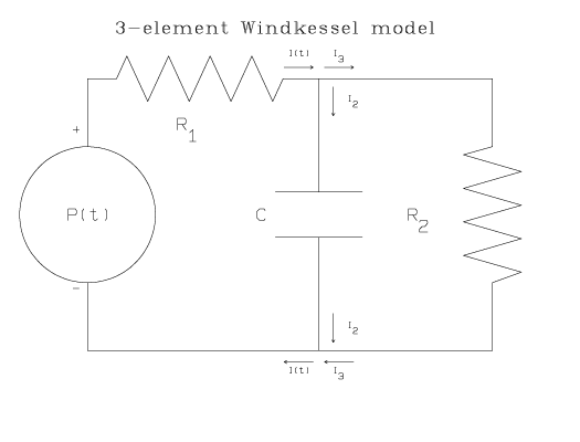
Using the same circuit analysis technique as for the 2-element Windkessel model circuit, the differential equation for the 3-element Windkessel model is found to be:
|
(3) |
where R1 represents the resistance due to the aortic valve or pulmonary valve, and R2 represents the peripheral resistance. I(t), P(t), and C have the same meanings as in the 2-element Windkessel equation.
Note that if R1 = 0 and R2 = R, the 3-element Windkessel equation reduces to the 2-element Windkessel equation. Also, during diastole when I(t) and its derivatives with respect to time are equal to zero, the solution of the 3-element Windkessel equation is:
|
(4) |
which is the same function, P(t), found for the 2-element Windkessel equation during diastole, if R2 = R.
Many modifications to the 2- and 3-element Windkessel models have been suggested. The electrical circuit corresponding to one such model that was used in studies of systemic circulation in chick embryo [17] and pulmonary circulation in the cat [13] and dog [7], resembles the 3-element Windkessel model, above, with a fourth inductor element added in the main branch of the circuit:
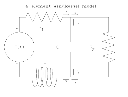
An inductor in the main branch of the circuit is said to simulate inertia of the fluid in the hydrodynamic model, which was neglected in the 2- and 3-element Windkessel models.
The drop in electrical potential across an inductor with inductance, L, is L [d I(t)/dt]. Following the circuit analysis method applied in the 2- and 3-element Windkessel models, one finds the following differential equation for this 4-element Windkessel model:
|
(5) |
In this equation, L has units of mass per length to the fourth power. Note that for L = 0, this 4-element Windkessel equation reduces to the 3-element Windkessel equation. Also, during diastole when I(t) and its derivatives vanish, we can solve for P(t) and get the same exponentially decreasing pressure function with decay time constant R2 C as in the 3-element Windkessel model.
The three Windkessel models described above, as well as any other Windkessel circuit analog, lead to an equation that relates blood pressure, blood flow, and various-order time derivatives thereof, via a set of parameters, such as (R, C), (R1, R2, C), and (R1, R2, C, L). Given a general equation such as (1), (3), and (5), there are three basic problems one can solve with MLAB:
As an example of how to solve the first problem with MLAB, suppose the blood flow to the aorta and pulmonary artery is given by:
|
||||||||||
where t is time in seconds from an agreed initial time, s is the period of the cardiac cycle in seconds, h is the length of time the aortic and pulmonary valves are open, in fractions of a second, during one cardiac cycle, and mod(t,s) denotes the remainder of t divided by s (i.e. mod(t,s) =t-ët/s ûs).
The following MLAB statements find the value of q0 such that the volume of blood for one cardiac cycle is 90 cubic centimeters, and then compute the time-course values for the aortic and pulmonary artery pressure during 3 cardiac cycles, assuming a 2-element Windkessel model equation with hemodynamic variables appropriate for a normal adult human. (Comments delimited by /* and */ are ignored by the MLAB interpreter.)
/* define normal human, hemodynamic constants in 2-element Windkessel model */
pl = 72 	/* cardiac cycles per minute */
s = 60/pl 	/* period of cardiac cycle in seconds */
h = (2/5)*s 	/* period of systole in seconds */
ml = 90 	/* blood output to aorta or pulmonary artery per
     cardiac cycle in cm^3 */

/* define function for blood flow as variable amplitude sine wave */
fct i(t,q0) = q0*sin(pi*t/h)

/* find peak amplitude of flow such that the total cardiac output is ml */
fct ampl() = root(z,0,1000,ml-integral(t,0,h,i(t,z)))
q0 = ampl()

/* define and compute flow for 3 cardiac cycles */
fct i1(t) = if ((tmd_mod(t,s))
The MLAB points operators invoke a numerical ordinary differential equation solver that uses the Adams method [13, pp. 740-744]. (MLAB also provides Gear and hybrid methods for solving ordinary differential equations, which may be more effective if the system of equations that is to be solved is stiff.)
The values of normal human peripheral resistance and arterial compliance for systemic and pulmonary arterial systems used above, were taken from Westerhof [15], and converted to the stated units using the fact that 760 mmHg = 1.0133 ×10⁶ dynes/cm2. By assigning other values to the parameters for peripheral resistance (r), arterial compliance (c), pulse (pl), period of systole (h), and volume of cardiac output (ml), this script can be used to find values of aortic and pulmonary artery pressure specified by the 2-element Windkessel model for a wide variety of conditions in humans or other animals.
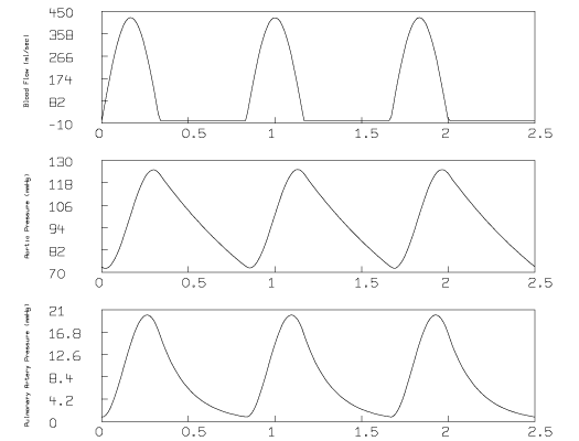
The flow function, aortic pressure, and pulmonary pressure curves can be graphed with the following additional MLAB commands:
draw af
left title "Blood Flow (ml/sec)" size .007
frame 0 to 1, .66 to .99
w1 = w
draw ms
left title "Aortic Pressure (mmHg)" size .007
frame 0 to 1, .33 to .66
w2 = w
draw mp
left title "Pulmonary Artery Pressure (mmHg)" size .007
frame 0 to 1, 0 to .33
view
The view command causes the graphs shown below to appear on the computer display:
The MLAB command:
plot in "wk.ps"can then be given to create a PostScript file named wk.ps that may be printed directly on a PostScript printer or inserted into a document using a word processor such as MS Word or WordPerfect.
While running the script above with different values for the initial pressure, p0, we noticed that the computed pressure function may not satisfy: P(0) = P(s); in other words, P(t) may not be periodic. This effect is evident in the following figure:
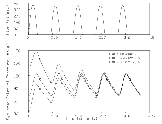
where there appears to be a decreasing trend underlying the oscillating pressure if P(0) is 145.7 mmHg, and an increasing trend underlying the oscillating pressure if P(0) is 36.4 mmHg.
The MLAB "FIT" statement can be used to enforce the periodic boundary condition, P(0) = P(s). This is done by inserting the following two statements in the script above, immediately before the statements involving the "points" operator:
fct f(t) = p(t)-p0
fit (p0), f to s&'0
The first statement defines the function f as the difference between the pressure at time, t, and the initial pressure. The second statement invokes the MLAB Levenberg-Marquardt least-squares fitting algorithm [14, pages 678-683] to find the value of the initial pressure, "p0", that best fits the data point (s,0), i.e. that imposes the boundary condition f(s) = 0.
As an example of how to solve the second problem with MLAB, suppose blood pressure measurements have been made through the course of a cardiac cycle and (time,pressure) ordered pairs have been stored in a file called press.dat. Then the following MLAB statements can be used to determine (time,flow) ordered pairs at the same times at which the pressure data was given, assuming the 2-element Windkessel model:
/* read (time,pressure)-ordered pairs from press.dat */
pdat = read(press,71,2) 	/* format = 71 rows, 2 columns */

/* define function for blood pressure as linear interpolation into pdat,
   and compute pressure for 1 cardiac cycle */
fct p(t) = lookup(pdat,t)
ap = points(p,0:pdat[71,1]!100)

/* define function for arterial flow under 2-element Windkessel model */
fct i(t) = p(t)/r+c*p't(t)

/* set r,c constants for systemic arterial system and compute aortic
   flow for 1 cardiac cycles */
r = .9000 		/* systemic peripheral resistance in (mmHg/cm^3/sec) */
c = 1.0666		/* systemic arterial compliance in (cm^3/mmHg) */
mi = points(i,0:pdat[71,1]!100)

/* draw aortic pressure and aortic flow */
draw ap
draw pdat lt none pt crosspt ptsize .005
left title "Aortic Pressure (mmHg)" size .01
no framebox
frame 0 to 1, 0 to .5
w1 = w
draw mi
left title "Aortic Flow (ml/sec)" size .01
frame 0 to 1, .5 to 1.
no framebox
view
The following graph results:
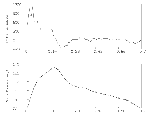
Note that there is considerable noise in the derived aortic flow curve. This is due to error and insufficient sampling in the pressure curve for times at the beginning of systole. The derived aortic flow depends on the time-derivative of p(t), which MLAB estimated numerically.
As an example of how to use MLAB to solve the third problem, we estimate 3- and 4-element Windkessel model parameters from data given by Molino, et. al., in reference [12]. Figure 1 of that reference presents graphs of aortic flow and aortic pressure during a cardiac cycle in a rat, and reports 2-parameter Windkessel model parameters for the rat's systemic circulation. We digitized the base aortic pressure and flow curves for the rat, and stored the resulting coordinates in a file called MOL.DAT. Then we used MLAB to:
(1) read the data file,
(2) solve the 2-element Windkessel model using Molino's reported peripheral
resistance and arterial compliance,
(3) find parameters for 3- and 4-element Windkessel models that minimize
the sum-of-squares,
(4) compute the Akaike Information Criterion (AIC) for each model, and
(5) graph the flow data, the pressure data, and the pressure curve
predicted by each model.
The values of the minimum sum-of-squares and the Akaike Information Criterion [1] are quantitative measures of how well a model fits a given data set; the lower the value, the better the fit.
/* read digitized from MOL.DAT: time in seconds in column 1, pressure in
   mmHg in column 2, flow in ml/sec in column 3. */
dt = read(mol,65,3)
n = nrows(dt) tv = dt
col 1 			/* time in seconds */
pdat = tv '(dt col 2) 	/* time,pressure ordered pairs */
idat = tv '(dt col 3) 	/* time,flow ordered pairs */

/* define flow function and evaluate for one cardiac cycle */
fct i1(t) = lookup(idat,mod(t,tv[n]))
af = points(i1,0:tv[n]!100)

/* define function for evaluating Akaike criterion given s=sum-of-squares,
   nd=number of data points, and np=number of parameters in model */
fct aic(s,nd,np) = nd*log(s)+2*np

/* 2-element Windkessel model with rw = peripheral resistance and
   cw = arterial compliance. Calculate values for parameters following
   Molino et al: peripheral resistance = mean pressure/mean flow;
   arterial compliance = time constant/peripheral resistance, where
   time constant = .529 seconds. */
fct pw't(t) = (i1(t)-pw(t)/rw)/cw
init pw(0) = pdat[1,2]
rw = mean(pdat col 2)/mean(idat col 2)
cw = .529/rw
mw2 = points(pw,0:tv[n]!100)
maxiter = 0
fit (cw), pw to pdat
a[1] = aic(sosq,n,2)
maxiter = 20

/* 3-element Windkessel model with rb1 = valve resistance, rb2 = peripheral
   resistance, and cb = arterial compliance */
fct pb't(t) = rb1*i1't(t)+((1+rb1/rb2)*i1(t)-pb(t)/rb2)/cb
init pb(0) = pdat[1,2]
rb1 = 0
rb2 = rw
cb = cw
fit (rb1), pb to pdat
a[2] = aic(sosq,n,3)
mb3 = points(pb,0:tv[n]!100)

/* 4-element Windkessel model with lm = inertial mass of fluid, rm1 = valve
   resistance, rm2 = peripheral resistance, and cm = arterial compliance. */
fct pm't(t)=lm*i1''t(t)+(rm1+lm/(cm*rm2))*i1't(t)+((1+rm1/rm2)*i1(t)-pm(t)/rm2)/cm
init pm(0) = pdat[1,2]
rm1 = rb1
rm2 = rb2
cm = cb
lm = 0 		/* in grams/cm^4 */
constraints q1 = {lm > 0}
fit (lm), pm to pdat constraints q1
a[3] = aic(sosq,n,4)
mm4 = points(pm,0:tv[n]!100)

/* draw graphs */
draw af
draw idat lt none pt circle ptsize .005
left title "Flow (ml/sec)" size .01
frame 0 to 1, .66 to .99
no framebox
w1 = w
draw mw2
draw mw2 row 1:100:15 lt none pt triangle ptsize .01
draw mb3
draw mb3 row 1:100:15 lt none pt square ptsize .01
draw mm4
draw mm4 row 1:100:15 lt none pt star ptsize .01
draw pdat
draw pdat row 1:n:2 lt none pt crosspt ptsize .01
left title "Pressure (mmHg)" size .01
title "Pressure data = +" at (.2,.85) ffract size .01
title "2-element = '27TC'R, AIC = "+a[1] at (.2,.8) ffract size .01
title "3-element = '27TB'R, AIC = "+a[2] at (.2,.75) ffract size .01
title "4-element = '27TE'R, AIC = "+a[3] at (.2,.7) ffract size .01
frame 0 to 1, 0 to .66
no framebox
view
plot in molwtp.ps
The resulting graph is:
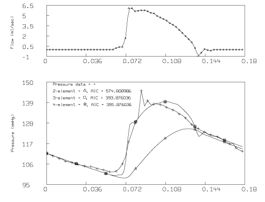
For the data from Molino, et.al, the parameters for the 2-element Windkessel model in a rat are 81.68 mmHg/cm3/sec for systemic peripheral resistance and 0.00648 cm3/mmHg for arterial compliance. The sum-of-squares for this model equals 8608.11 and the Akaike Information Criterion equals 574.8. The value for systemic peripheral resistance is a thousand times greater than the value for a human, and the value of arterial compliance is a thousand times less than the value for a human.
The value found by the statement fit (rb1), pb to pdat for the aortic valve resistance in the 3-element Windkessel model, equals 4.285 mmHg/cm3/sec. The sum-of-squares value of 471.9 and the Akaike Information Criterion value of 393.9 indicate that this 3-element Windkessel model is a better model for this data than the 2-element Windkessel model. From the graph, it is clear that this improvement arises primarily in the systole part of the cardiac cycle.
The value found by the statement fit (lm), pm to pdat constraints q1 for the inductance in the 4-element Windkessel model is 0. The constraint q1 was necessary to prevent the value of lm from becoming negative. The sum-of-squares value of 471.9 and the Akaike Information Criterion value of 395.9 indicate that the 4-element Windkessel model does not provide a significant improvement over the 3-element Windkessel model.
The MLAB scripts above demonstrated how to obtain pressure or flow curves for the 2-,3-, and 4-element Windkessel models. It is a simple matter to obtain pressure or flow curves for any other differential model. Once the differential equation has been derived by analysis of an hydraulic or electrical circuit, simply: 1) re-arrange the differential equation so that the highest order derivative of the desired curve (P(t) or I(t)) is alone on the left side of the equation (say this is the nth-order derivative); 2) write an MLAB function definition statement for the highest time-derivative of the desired curve (a jth-order derivative with respect to time is expressed by typing the function name, followed by j apostrophes, followed by t(t)); 3) add an MLAB initial condition statement, such as init p''t(0) = 800, for each jth-order derivative, where j = 1,2,...,(n-1); 4) add an assignment statement with an appropriate value for each parameter in the model; 5) define the known function (I(t) or P(t)); and 6) use the points operator to solve for the desired curve.
Related problems one can solve with MLAB:
The Windkessel models described above assume constant values for peripheral resistance and arterial compliance. Apter [2] noted that the assumption of constant peripheral resistance is not justifiable since carotid sinus baroreceptors are stimulated in late systole and early diastole and they change the peripheral resistance. One could, for example, accomodate variable peripheral resistance in the 2-element Windkessel model by using the following MLAB statements to define the derivative of pressure with respect to time:
/* define function for the derivative of the pressure, but use
   a function for resistance, rather than a constant */
fct p't(t) = (i1(t)-p(t)/r(t))/c

/* define the function for variable resistance */
fct r(t) = r0-g*(p(t-tau)-ps0)
The definition of the function r(t) in this example would accomodate delays in the pressure, much as Apter described in her paper.
Similarly, Fogliardi [5] cited constant arterial compliance as a limitation in the 3-element Windkessel model and proposed introducing a non-linear function of pressure for the constant arterial compliance. A non-linear function of pressure for arterial complaince could be introduced in the 3-element Windkessel as follows:
/* define function for the derivative of the pressure, but use a
   function for capacitance, rather than a constant */
fct p't(t) = r1*i1't(t)+((1+r1/r2)*i1(t)-p(t)/r2)/c(t)

/* define an exponential function for variable capacitance */
fct c(t) = a*exp(b*p(t))
Another way in which variable arterial compliance in the Windkessel model might be introduced is by including higher order terms in pressure. The derivation of the 2-element Windkessel equation assumed the air pressure and volume were related by [dP/dV] = C or P(t) = CV(t). One could derive a different equation by assuming a non-linear relation between P and V, such as PV = constant, which would hold for an ideal gas, and solve that equation with MLAB.
Karamanoglu [8] describes a method for measuring pressure curves away from the aorta, for example at the brachial artery. MLAB includes signal analysis functions which could be used to derive the aortic pressure curve given the remote pressure curve and appropriate transfer function. With simultaneous EKG and pressure curves, one could use MLAB to develop models for the electrical activity of the heart.
Another research question is: are there chaotic trajectories for Windkessel differential equations? Such behavior would be useful in understanding arrythmias.
References:
1. Akaike, H., ``A new look at the statistical model identification'', IEEE Trans. Automat. Contr. AC-19 (1974) 716-723.
2. Apter, Julia T., ``An Analysis of the Aortic Pressure Curve During Diastole'', Bull. Math. Biophys. 25 (1963) 325-339.
3. Broemser, Ph., et. al., ``Ueber die Messung des Schlagvolumens des Herzens auf unblutigem Weg'', Zeitung für Biologie 90 (1930) 467-507.
4. Dinnar, Uri, Cardiovascular Fluid Dynamics (Boca Raton, FL: CRC Press, 1981), pp. 139-147.
5. Fogliardi, Roberto, et.al., ``Comparison of linear and nonlinear formulations of the three-element windkessel model'', Am. J. Physiol. 271 (1996) H2661-H2668.
6. Frank, Otto, ``Die Grundform des arteriellen Pulses'', Zeitung für Biologie 37 (1899) 483-586.
7. Grant, B.J.B., et.al., ``Characterization of pulmonary arterial input impedance with lumped parameter models'', Am. J. Physiol. 252 (1987) H585-H593.
8. Karamanoglu, Mustafa, ``A System for Analysis of Arterial Blood Pressure Waveforms in Humans'', Computers and Biomedical Research 30 (1997) 244-255.
9. Kenner, Thomas, ``Chapter 2: Physical and Mathematical Modeling in Cardiovascular Systems'' appearing in Quantitative Cardiovascular Studies, Clinical Research Applications of Engineering Principles, ed. by Ned Hwong, D.R.Gross, D.J.Patel, (Baltimore, MD: University Park Press, 1979) pp. 41-109.
10. Lambermont, B., et.al., ``Comparison between Three- and Four-Element Windkessel Models to Characterize Vascular Properties of Pulmonary Circulation'', Arch. Physiol. and Biochem. 105 (1997) 625-632.
11. Lieber, B.B., et.al., ``Beat-by-Beat changes of viscoelastic and inertial properties of the pulmonary arteries'', J. Appl. Physiol. 53 (1994) 2348-2355.
12. Molino, Paola, et.al.,``Beat-to-beat estimation of windkessel model parameters in conscious rats'', Am. J. Physiol. 274 (1998) H171-H177.
13. Piene, H., et.al., ``Does normal pulmonary impedance constitute the optimum load for the right ventricle?'', Am. J. Physiol. 242 (1982) H154-H160.
14. Press, W.H., et.al., Numerical Recipes in Fortran: The Art of Scientific Computing, (Cambridge University Press: NY, 1992).
15. Westerhof, Nicolaas, et.al., ``An artificial arterial system for pumping hearts'', Journal of Applied Physiology 31 (1971) 776-781.
16. Yoshigi, Masaaki, et.al., ``Dorsal aortic impedance in stage 24 chick embryo following acute changes in circulating blood volume'', Am. J. Physiol. 270 (1996) H1597-H1606.
17. Yoshigi, Masaaki, et.al., ``Characterization of embryonic aortic
impedance with lumped parameter models'', Am. J. Physiol. 273 (1997)
H19-H27.