Minimal Models for Glucose and Insulin Kinetics

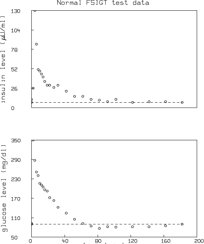
Qualitatively, the glucose level in plasma starts at a peak due to the injection, drops to a minimum which is below the basal (pre-injection) glucose level, and then gradually returns to the basal level. The insulin level in plasma rapidly rises to a peak immediately after the injection, drops to a lower level which is still above the basal insulin level, rises again to a lesser peak, and then gradually drops to the basal level. Depending on the state of the subject, there can be wide variations from this response; for example, the glucose level may not drop below basal level, the first peak in insulin level may have different amplitude, there may be no secondary peak in insulin level, or there may be more than two peaks in insulin level.
The glucose and insulin minimal models provide a quantitative and parsimonious description of glucose and insulin concentrations in the blood samples following the glucose injection. The glucose minimal model involves two physiologic compartments: a plasma compartment and an interstitial tissue compartment; the insulin minimal model involves only a single plasma compartment. The glucose and insulin minimal models allow us to characterize the FSIGT test data in terms of four metabolic indices:
This paper will demonstrate the use of the mathematical modeling computer program MLAB to simulate insulin and glucose plasma levels during an FSIGT test and determine values of the metabolic indices from a data set via curve-fitting.
Reference 3 provides the following FSIGT test data (also shown in the graphs above) from a normal individual:
| time (minutes) | glucose level (mg/dl) | insulin level (mU/ml) |
| 0 | 92 | 11 |
| 2 | 350 | 26 |
| 4 | 287 | 130 |
| 6 | 251 | 85 |
| 8 | 240 | 51 |
| 10 | 216 | 49 |
| 12 | 211 | 45 |
| 14 | 205 | 41 |
| 16 | 196 | 35 |
| 19 | 192 | 30 |
| 22 | 172 | 30 |
| 27 | 163 | 27 |
| 32 | 142 | 30 |
| 42 | 124 | 22 |
| 52 | 105 | 15 |
| 62 | 92 | 15 |
| 72 | 84 | 11 |
| 82 | 77 | 10 |
| 92 | 82 | 8 |
| 102 | 81 | 11 |
| 122 | 82 | 7 |
| 142 | 82 | 8 |
| 162 | 85 | 8 |
| 182 | 90 | 7 |
Using a spreadsheet program, word processor, or the MLAB file edit command directly, these numbers can be stored in an ASCII text file named "TEST.DAT".
The following diagram summarizes the minimal model for glucose kinetics:
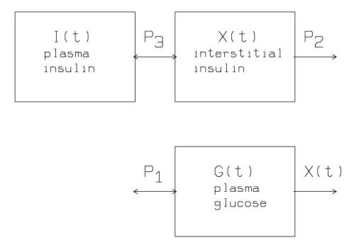
Insulin leaves or enters the interstitial tissue compartment at a rate proportional to the difference between the plasma insulin level, I(t), and the basal level, Ib; if the plasma insulin level falls below the basal level, insulin leaves the interstitial tissue compartment, and if the plasma insulin level rises above the basal level, insulin enters the interstitial tissue compartment. Insulin also disappears from the interstitial tissue compartment via a second pathway at a rate proportional to the amount of insulin in the interstitial tissue compartment.
Glucose leaves or enters the plasma compartment at a rate proportional to the difference between the plasma glucose level, G(t), and the basal level, Gb; if the plasma glucose level falls below the basal level, glucose enters the plasma compartment, and if the glucose level rises above the basal level, glucose leaves the plasma compartment. Glucose also disappears from the plasma compartment via a second pathway at a rate proportional to the amount of insulin in the interstitial tissue.
The differential equations corresponding to the glucose minimal model are:
| |||||||||||||||
with G(0) = G0 and X(0) = 0. In these equations, t is time, G(t) is the plasma glucose concentration at time t, I(t) is the plasma insulin concentration at time t, and X(t) is the interstitial insulin at time t. Gb is the basal plasma glucose concentration and Ib is the basal plasma insulin concentration. Basal plasma concentrations of glucose and insulin are typically measured either before, or 180 minutes after, administration of glucose. There are four unknown parameters in this model: p1, p2, p3, and G0.
Note that in this model, glucose is utilized at the constant rate p1, when we neglect feedback effects due to interstitial insulin as represented by the term -X(t) ·G(t). An additional amount of plasma insulin will cause the amount of interstitial insulin to change, which in turn, will cause the rate of glucose utilization to change. The insulin sensitivity is defined as SI = p3/p2 and the glucose effectiveness is defined as SG = p1.
The following MLAB commands in the do-file "g.do" estimate values for the parameters p1, p2, p3, and G0 given the time course of plasma glucose and insulin. The values of the parameters found minimize, in the least squares sense, the weighted difference between the measured time course of plasma glucose and the parameter-dependent solution to the glucose minimal model differential equations. The plasma insulin concentration function is obtained by linear interpolation of the time-insulin values listed in TEST.DAT. This is done by employing the MLAB function "LOOKUP".
"file: g.do = glucose minimal model"
"-------"
"get data consisting of time values in column 1, plasma glucose"
"levels in column 2, and plasma insulin levels in column 3. Set"
"n to the number of time values. Set gdat to the (time,glucose level)"
"ordered pairs. Set idat to the (time,insulin level) ordered pairs."
data = read(test,50,3);
m = nrows(data);
gdat = data col (1,2);
idat = data col (1,3);
"define the glucose minimal model:"
" t is time"
" g(t) is plasma glucose level"
" i(t) is plasma insulin level, empirically-defined by interpolation in idat"
" x(t) is interstitial insulin"
" gb is basal (180 min) plasma glucose level"
" ib is basal (180 min) plasma insulin level"
fct g't(t) = -(p1+x(t))*g(t)+p1*gb
fct x't(t) = -p2*x(t)+p3*(i(t)-ib)
fct i(t) = lookup(idat,t)
init g(0) = g0
init x(0) = 0.0
gb = gdat(m,2) ib =
idat(m,2)
"define weights for glucose level data, censoring data up to time t = 8"
fct wf(i) = if gdat(i,1) < 8 then 0 else if gdat(i,1) = 8 then 10 else 1
wts = wf on 1:m
"define constraints for p1, p2, p3, and g0"
constraints q = {p1>0,p2>0,p3>0,g0>0}
"give initial estimates for parameters p1,p2,p3, and g0"
p1 = .03082; p2 = .02093; p3 = .00001062; g0 = 287;
"fit the model to the weighted data with defined constraints"
fit (p1,p2,p3,g0), g to gdat with weight wts constraints q
type "glucose effectiveness",p1
type "insulin sensitivity",p3/p2
"draw 3 graphs:1-plasma insulin level function and data vs time"
" 2-interstitial insulin vs time"
" 3-fitted glucose level function and data vs time"
"horizontal dashed lines show basal levels"
top title "GLUCOSE MINIMAL MODEL"
draw idat pt circle ptsize .01
draw shape(2,2,list(idat(1,1),ib,idat(m,1),ib)) lt dashed pt circle ptsize .01
left title " insulin level ('15Tm'RU/ml)"
delete w.xaxis
frame .25 to .75, .667 to 1
w1 = w
draw points(x,gdat(1,1):gdat(m,1)!200)
left title �nterstitial insulin"
delete w.xaxis
frame .25 to .75, .334 to .666
w2 = w
draw points(g,gdat(1,1):gdat(m,1)!200)
draw gdat lt none pt circle ptsize .01
draw shape(2,2,list(gdat(1,1),gb,gdat(m,1),gb)) lt dashed pt circle ptsize .01
left title "glucose level (mg/dl)"
bottom title "time v(min)"
frame .25 to .75, 0 to .333
view
save idat,gdat,ib,gb,g0,m in tmp.sav
The MLAB log-file and picture generated by executing the do-file "g.do" follow:
* do "g.do"
final parameter values
    value 	     error 	 dependency 	parameter
0.02649256302 	0.01367779755 	0.9976038298 	   P1
0.02543609572   0.029223424     0.9932825935       P2
1.281692067e-05 1.516217536e-05 0.9978008452 	   P3
279.1123014     15.38803832     0.9901777503       G0
5 iterations
CONVERGED
best weighted sum of squares = 4.237885e+02
weighted root mean square error = 4.603197e+00
weighted deviation fraction = 1.469631e-02
R squared = 6.905055e-01
no active constraints

	glucose effectiveness
P1 = .026492563

	insulin sensitivity
       = 5.03887106E-4

creating save file: TMP.SAV
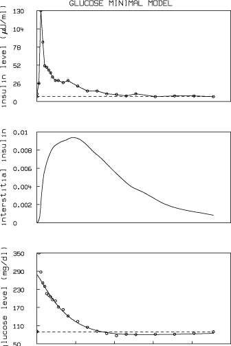
The insulin sensitivity, SI, for this data set is estimated as 5.039 ×10⁻⁴ min-1 ·(mU /ml)-1 which is within the normal range reported in reference 2: 2.1 to 18.2 ×10⁻⁴ min-1 ·(mU / ml)-1. The glucose utilization, SG, for this data set is estimated as 0.0265 min-1, which is also within the normal range reported in reference 2: 0.0026 to 0.039 min-1.
Next we examine the minimal model for insulin kinetics.
The following diagram summarizes the minimal model for insulin kinetics:
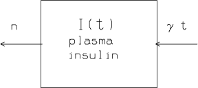
The course of plasma glucose in time, G(t), is given by linear interpolation of the time-glucose values listed in TEST.DAT. Insulin enters the plasma insulin compartment at a rate proportional to the product of time and the concentration of glucose above a threshold amount. Here, time is the interval, in minutes, from the glucose injection. If the plasma glucose level drops below the threshold amount, the rate of insulin entering the plasma compartment is zero. Insulin is cleared from the plasma compartment at a rate proportional to the amount of insulin in the plasma compartment.
The minimal model for insulin kinetics is given by the equation:
| ||||||||||||
with I(0) = I0. n is the insulin clearance fraction, h is roughly the basal glucose plasma level, and g is a measure of the secondary pancreatic response to glucose. The first phase pancreatic responsivity is defined as f1 = (Imax-Ib)/[n·(G0-Gb)] where Imax is the maximum insulin response. The second phase pancreatic responsivity is defined as f2 = g×104.
The following MLAB commands in the do-file GI.DO estimate values for the parameters n, g, h, and I0 given the time course of plasma glucose. The values of the parameters found minimize (in the weighted least squares sense) the difference between the measured time course of plasma insulin and the parameter-dependent solution to the insulin minimal model differential equations.
"file: gi.do = insulin minimal model"
reset

"read insulin, glucose levels from temporary save file"
use tmp.sav

"define the insulin minimal model"
fct i't(t) = -n*i+gama*(if g(t) < h then 0 else (g(t)-h))*t
fct g(t) = lookup(gdat,t)
init i(0) = i0

"determine weights for insulin data"
fct wf(i) = if idat(i,1) < 3 then 0 else if idat(i,1) <= 8 then 10 else 1
wts = wf on 1:m

"define a constraint set for all the parameters"
constraints q1 = {n > 0, gama > 0, h > 0, i0 > 0}

"provide initial guesses for the paramters"
n = .3; gama = .003349; h = 89.50; i0 = 410.4

"fit the insulin minimal model to the insulin data"
DISASTERSW = -1
fit (n,gama,h,i0), i to idat with weight wts constraints q1

type "phase 1 pancreas responsivity",(maxv(idat)-ib)/(n*(g0-gb)) type
"phase 2 pancreas responsivity",10000*gama

"draw 2 graphs:1-fitted plasma insulin level and data vs time"
"     2-glucose plasma level data vs time"
top title "INSULIN MINIMAL MODEL"
draw idat lt none pt circle ptsize .01
draw points(i,idat(1,1):idat(m,1)!100)
draw shape(2,2,list(idat(1,1),ib,idat(m,1),ib)) lt dashed pt circle ptsize .01
left title " insulin level ('15Tm'RU/ml)"
delete w.xaxis
frame .15 to .85, .5 to 1
w1 = w

draw gdat pt circle ptsize .01
draw shape(2,2,list(gdat(1,1),gb,gdat(m,1),gb)) lt dashed pt circle ptsize .01
left title "glucose level (mg/dl)"
bottom title "time v(min)"
frame .15 to .85, 0 to .5
view
The log-file and picture generated by executing the do-file GI.DO follow:
* do "gi.do"
Using: M,G0,GB,IB,GDAT,IDAT
final parameter values
    value 	     error 	 dependency 	parameter
0.2673230345 	0.01603033225 	0.9611152205        N
0.004074459794  0.0006378976592 0.7211259427      GAMA
83.74403736 	2.329398193 	0.2073681454 	    H
363.666326 	26.5919455 	0.9471979611       I0
4 iterations
CONVERGED
best weighted sum of squares = 1.292680e+03
weighted root mean square error = 8.039529e+00
weighted deviation fraction = 2.772192e-02
no active constraints

	phase 1 pancreas responsivity
       = 3.46163989
	phase 2 pancreas responsivity
       = 40.7445979
Note that when performing the least squares minimization between the solution of the insulin minimal model equation and the measured plasma insulin levels, relative weights of 0, 10, and 1, were assigned to the plasma insulin levels so that less reliable values would not adversely effect the estimation of parameters and more reliable values would be more heavily weighted. Using appropriate weights is generally important in fitting forms of the minimal model. While there are many ways of weighing data, this particular method was suggested by Walton (reference 6).
The glucose minimal model provides differential equations for the plasma glucose and interstitial insulin levels. The insulin minimal model provides a differential equation for the plasma insulin level. It is possible to combine all three differential equations into one model. This is demonstrated in the following do-file, GGI.DO:
"file: ggi.do - combined glucose and insulin minimal models"
"read insulin, glucose levels from temporary save file"
use tmp.sav

"define the combined glucose-insulin minimal model"
fct i't(t) = -n*i+gama*(if g < h then 0 else (g-h))*t
fct g't(t) = -(p1+x)*g+p1*gb
fct x't(t) = -p2*x+p3*(i-ib)
init i(0) = i0
init g(0) = g0
init x(0) = 0

"determine weights for glucose level data, censoring data up to time t = 8"
fct wg(i) = if gdat(i,1) < 8 then 0 else if gdat(i,1) = 8 then 10 else 1
wgs = wg on 1:m

"determine weights for insulin level data"
fct wi(i) = if idat(i,1) < 3 then 0 else if idat(i,1) <= 8 then 10 else 1
wis = wi on 1:m

"define a constraint set for all of the parameters"
constraints q1 = {n>0,gama>0,h>0,p1>0,p2>0,p3>0,i0>0,g0>0}

"provide initial guesses for the parameters"
n = .3; gama = .003349; h = 89.50; p1 = .03082; p2 = .02093
p3 = .00001062; i0 = 403.4; g0 = 287

"fit both of the models to the data"
disastersw = -1
fit (n,gama,h,p1,p2,p3,i0,g0), i to idat with weight wis, \
   g to gdat with weight wgs, constraints q1

type "glucose effectiveness",p1
type "insulin sensitivity",p3/p2
type "phase 1 pancreas responsivity",(maxv(idat)-ib)/(n*(g0-gb))
type "phase 2 pancreas responsivity",10000*gama
Here is the resulting MLAB log-file and picture:
final parameter values
    value            error 	 dependency 	parameter
0.2658844452 	0.01153178897 	0.9621356273 	    N
0.003911687955 	0.0004693022146 0.7457248671      GAMA
79.03532257     2.421480638 	0.4908060854        H
0.03168360775 	0.004806175221 	0.9712465296 	   P1
0.0123362991 	0.006558350386 	0.888606309        P2
4.891692162e-06 1.923309135e-06 0.9627481277 	   P3
364.8353065 	18.88965714 	0.9496151759       I0
291.2242018 	5.82052435 	0.8836723395 	   G0
5 iterations
CONVERGED
best weighted sum of squares = 1.278572e+03
weighted root mean square error = 5.653697e+00
weighted deviation fraction = 1.545963e-02
R squared = 3.943754e-01
no active constraints

	glucose effectiveness
	P1 = 3.16836078E-2

	insulin sensitivity
	= 3.96528337E-4

	phase 1 pancreas responsivity
	= 3.27088221

	phase 2 pancreas responsivity
	= 39.1168796
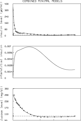
These results show that, as is common, there is not a unique set of parameters that characterize a FSIGT test data set. The combined minimal model is seen to generate slightly lower values for glucose effectiveness and insulin sensitivity than the glucose minimal model, and slightly higher values for phase 1 and 2 pancreas responsivity than the insulin minimal model.
There are various devices that could be explored in order to improve the family of models studied here. First, these models employed the MLAB operator "LOOKUP" to linearly interpolate glucose and insulin plasma time course data. Alternatively, the MLAB operator "SMOOTHSPLINE" could be used to provide glucose and insulin plasma time course curves that are not only continuous, but also have continous first and second derivatives.
Second, several authors have augmented the insulin minimum model to account for plasma levels of C-peptide (see references 7-9). It is a straightforward exercise to implement the C-Peptide minimal model using MLAB.
This paper has shown how MLAB can be used to calculate diagnostically important metabolic indices which arise in the glucose and insulin minimal models from frequently-sampled intravenous glucose tolerance test data. The MLAB program is generally an ideal tool for the study of compartmental models. You can contact Civilized Software for further examples in neurophysiology and pharmacology.
References: