Supply Forecasting via Survival Curve Estimation
Suppose we have "shelf-life'' data for a group of n items. These items might be automobiles, or laser printer toner cartridges, or vials of vaccine, or entry-slots for admission to a course. In the case of a physical item which is to be replaced as it is "consumed'', we are interested in forecasting the nature and rate of consumption, and in estimating a suitable replacement schedule. This is an important component of planning and managing the supply-logistics for the items of interest.
Suppose, that for most items, we have the age of the item when it was "consumed'', i.e. removed from our group of items; this age is the "shelf-life'' of that item; generally this age is called the survival time of the item. However, let us also suppose we may have censoring present; that is, for some consumed items, we do not have the exact survival time, i.e. the exact age at consumption, but only an age for the item such that at some unknown time after this age, the item was consumed. In this case, the actual survival time has been "censored'', i.e. hidden from our view. This kind of complication might arise when, for example, incomplete records are kept, or when dates of consumption are not recorded consistently, but periodic inventory data is available.
Our data thus consists of pairs of values (y1,e1), (y2,e2), ..., (yn,en) where each ei is either 0 or 1. When ei = 1, yi is the survival time until the consumption of item i, counting from the study starting point, and when ei = 0, yi is the censoring time for item i, indicating that item i was lost to follow-up with an unknown consumption time sometime after yi time-units from the study starting point. The value ei is called the result-code for item i.
Suppose the items in the group being studied have survival times, X1, X2, .... Xn, which are independent identically-distributed random variables, a realization of which is, except for censoring, given by our data. Let F(t) be the common distribution function of X1, ..., Xn. We wish to estimate the survival function S(t) = P(Xi > t) = 1-F(t).
Associated with each Xi, we postulate a censoring-time random variable, Ci. The random variables C1, ..., Cn are assumed to be independent and identically-distributed, with the distribution function G(t) = P(Ci Ł t). For any realization, ([X^]i,[C^]i) where [X^]i is a sample of Xi and [C^]i is a sample of Ci, if [X^]i Ł [C^]i, we have yi=[X^]i, and ei = 1, while when [X^]i > [C^]i, we have yi=[C^]I and ei = 0. Thus, the value yi is a sample of min(Xi,Ci).
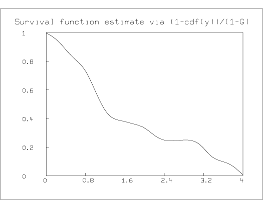
If we assume a specific formula for the censoring-time distribution function G(t), then we can estimate S(t) by (1-H(t))/ (1-G(t)) where H(t) is the empirical cumulative distribution function of the data-values y1, ..., yn. It is appropriate to adjust this estimate to be monotonically-decreasing and to smooth it to obtain the final estimate. For example, suppose the censoring-time distribution is uniform on the interval [0,4]; then, given the column vector Y listed below, where Yi holds the observed survival time yi, we can estimate the survival function S in MLAB with the function SE given below, and then monotonize, smooth, and graph it. The actual result-code vector, E, associated with this data is listed below together with Y for later reference, even though E is not needed to be used in the parametric estimating function SE.
*TYPE Y&'E

MATRIX :
1.635686	0
.3113416	0
.4963642	1
1.131409	0
2.221448	0
1.668752	1
2.785097	0
.3379156	0
.4495545	1
3.020983	1
.3994093	0
.9359379	1
.9697097	0
.6193121	0
.1234482	0
.8931070	1
.2233199	1
.8303535	0
3.926499	0
2.012626	1
.3871494	1
.9381460	1
1.210837	1
1.704919	0
1.006140	1
1.998524	1
.3763392	0
1.184550	0
.7832847	1
.9971150	0
.0452861	0
2.145687	1
.8396369	1
1.319498	0
3.288359	1
.7552886	1
1.017174	0
.8238844	1
.5893285	1
.2916714	0
3.266290	0
2.215458	1
.5546782	0
.1355474	1
.1247086	0
.9045237	1
.4080161	1
1.188316	1
1.243582	1
1.043640	1


*L = 4
*H = CDF(Y)
*FUNCTION SE(T)=IF T>=L THEN 0 ELSE (1-LOOKUP(h,t))/(1-T/L)
*DRAW SMOOTHSPLINE(MONOT(POINTS(SE,0:L:.1), -1), 0:L!140)
*top title "Survival function estimate via (1-cdf(y))/(1-G)"
*VIEW

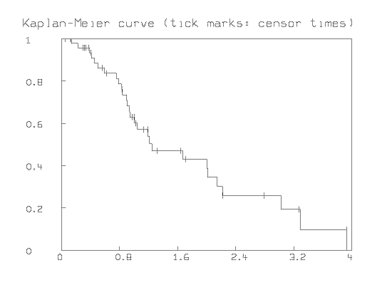
We can avoid assuming a specific censoring-time distribution by using the asymptotically-unbiased Kaplan-Meier product-limit estimator function, [S^] as the estimator function for the survival function S. This can be computed in MLAB using the KMSURV function and graphed using the STEPGRAPH function.
For example, given the data vector, Y, listed above, together with the associated result-code vector, E, we can produce a graph of our estimated survival curve [S^] as shown below. The tic-marks show the points where censored observations occur.
*DELETE W
*D = Y&'E
*D = SORT(SORT(D,2,-1),1)
*H1 = KMSURV(D)
*H = STEPGRAPH(H1 COL 1:2)
*R = (0 &' 1) & H & H[NROWS(H),1]&' 0)
*DRAW R, COLOR RED
*Y1 = COMPRESS(D,2,1) COL 1
*FCT F(X) = LOOKUP(H,X)
*H2 = POINTS(F,Y1)
*DRAW H2 LINE NONE, PT VBAR, PTSIZE .015, COLOR GREEN
*WINDOW 0 TO 4, 0 TO 1
*TOP TITLE "Kaplan-Meier curve (tick marks: censor times)"
*VIEW
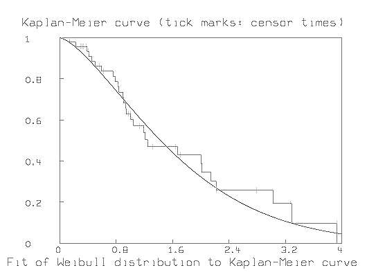
We may postulate a specific form for the distribution of the Xi random variables. For example, if the survival time distribution function is a Weibull distribution with group-specific parameters, a and b, then the survival curve is given by SW(t) = exp(-(t/a)b).
Now, we may estimate the parameters a and b using MLAB to fit the model function SW(t) to a matrix of points lying on the Kaplan-Meier estimated survival curve. This is demonstrated for the matrix H1 of points on the estimated survival curve obtained above. Greenwood's variance approximation for [S^] computed by KMSURV() in H1 col 3 is used to compute appropriate weights for the curve-fit.
*FUNCTION SW(T)=EXP(-((IF T=0 THEN .000001 ELSE T)/A)^B)
*A = 1;B = 1; H1[1,3] = 1
*FIT(A,B), SW TO H1 COL 1:2 WITH WEIGHT 1/(H1 COL 3)
final parameter values
   value            error             dependency    parameter
    1.837800012    0.05250877741     0.3849266596   A
    1.451240067    0.05755968774     0.3849266596   B
4 iterations
CONVERGED
best weighted sum of squares = 8.691990e+00
weighted root mean square error = 5.673848e-01
weighted deviation fraction = 1.869069e-02
R squared = 9.756895e-01
*DRAW POINTS(SW,0:4:.05)
*bottom title "Fit of Weibull distribution to Kaplan-Meier curve"
*view
Sometimes we may wish to compare the survival curves of several dissimilar groups of items, to determine, for example, which of several distinct marketing strategies is superior. This can be done by comparing the estimated survival curves directly with an appropriate statistical test (such as the Mantel-Haensel test, MHT) provided by MLAB.
It may be of interest to compute the expected survival time of an
item that has already survived k time-units, i.e. has not
been consumed by time k. This is just
M(k):=ňkĄ tq(t|k) dt,
where q(t | k) is the conditional density function, d[P(X1 ł t |X1 ł k)]/dt. But given the survial time distribution function F and
the corresponding density function f(t) = dF(t)/dt, we can compute q(t| k) = if t < k then 0 else f(t)/a, where
|
Note q(t | 0) = 0 and q(t|t) is just the hazard function f(t)/S(t).
The expected additional survival time function M(k) can be easily computed and graphed in MLAB. One use for the function M(k) is to estimate lifetimes for items with censored survival times. By thus "completing'' a data set, we obtain uncensored data which is amenable to a variety of otherwise inapplicable statistical procedures.
Now we may suppose we have a survival function s(t), possibly obtained by curve-fitting observed survival data, that describes the survival time characteristics of the items of interest. Thus, we assume we have the survival function s, where s(t) is the fraction of items which survive at least to time t. Suppose that we wish to replace these items on a regular schedule so as to maintain the constant level of a0 items available. It is reasonable to assume that each newly-introduced replacement batch of items follows the same survival behavior as the original items. We wish to compute the replacement schedule function. Note the replacement function can be used for budget projection purposes.
Here we shall look at the discrete formulation of the problem where time
is measured in discrete increments as an integer value of say,
hours, days or weeks. Set
s0 = 1 and in general let si be the fraction of items which
survive for at least i weeks. Let a0 be the initial number of
items at time 0, and let ai denote the number of items
available at the beginning of week i.
Then the number of these items available at the start of
week k is a0sk+a1sk-1+Ľ+aks0. Since we wish to
maintain the constant level of a0 items at each week, we equate a0
and a0sk+a1sk-1+Ľ+aks0.
From this we get the following recursion
equation for ak, 0 Ł k.
|
This represents the solution vector of the following lower-triangular Toeplitz system.
|
The MLAB function DECONV may be used to compute the solution to this linear system.
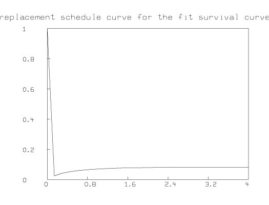
For example, here is the replacement schedule function computed by using DECONV based on the best-fitting Weibull survival curve for the data above. Note the first point indicates we obtain the entire initial group of items at once (100 percent). Note also that the replacement schedule curve rapidly converges to a nearly-constant replacement amount per week.
In practice, we should re-estimate our survival curve and replacement schedule curve from time to time, so that changes in consumption do not invalidate the resupply process.