The study of how a ligand material, such as a hormone or antibody, binds to one or more kinds of molecular complexes, called sites, is of fundamental importance in biochemistry. Sites are often embedded in cell membranes, and the binding serves to control the behavior of the cell itself. Typically we are interested in the number of distinct kinds of sites and their frequency of occurrence, and also the equilibrium constants for each ligand-site binding reaction which indicates the absolute strength of each such binding reaction.
For example, quantitative analysis of hormone-receptor binding can be easily performed using appropriate software such as MLAB. MLAB is a computer program whose name is an acronym for "modeling laboratory"; it is an interactive system for mathematical modeling, originally developed at the National Institutes of Health. MLAB can fit multiple non-linear models to data points obtained from standard direct-binding or competitive displacement assays. Typical assays involve measuring the competition between radiolabelled and cold ligand in detergent-solubilized membrane preparations or on whole cells. Affinity constants and limit values of binding protein concentrations for single or multiple sites can be computed by fitting saturation curves in MLAB. Output can include Scatchard plots obtained by a suitable transformation.
There are two common categories of data. The first category results from cold displacement of bound labeled ligand where the labelled ligand concentration is held constant, the unlabelled ligand concentration is varied, and the ligand binding is calculated as a function of the proportion of labelled to total ligand concentration. The second category is a straight saturation analysis where the ligand binding is measured as a function of increasing labelled ligand concentration. This latter category of data also arises in fluorescent, ultraviolet, or electrical current studies. In general, MLAB can handle any measurements modeled by linear or nonlinear saturation plots.
In practice, the basic data must be adjusted to account for an experimentally-determined nonspecific binding level, specific activity of the labelled ligand, the values for maximal binding of the cellular preparations, and defective non-binding ligand. Replicate data points need not be averaged; they are entered as individual data points which are each included in the curve fitting process. In contrast, curve fitting based on dose averages may require careful attention to weights to obtain a reasonable fit. Experimental researchers rarely have a priori knowledge of the validity of individual data points, so each point is generally assigned an unbiased equal weight. However, weighting functions can be differentially applied in MLAB to adjust for differing error percentages, such as may occur in measurements of low levels of radioactivity. Because of the options for flexible weights, MLAB addresses some of the problems inherent in the treatment of experimental data where the number of samples is usually low and the error can be relatively high.
MLAB can be used to analyze down and up regulation in receptor number on the cell surface, where the binding capacity or receptor concentration is the limiting -intercept on the Scatchard plot. The MLAB program is also useful in determining whether changes in binding by different ligand agonists/antagonists can be attributed to reduced binding affinity of the defined site/sites (seen as changes in the affinity constant), or to the total loss of binding ability of a class of sites (seen as changes in the binding capacity, and changes in the fit from an to site model). Similarly, MLAB can aid in comparison studies of a single ligand against different binding proteins that vary by site-directed mutagenesis, or alternative splicing; such analyses can be useful in exploring mechanisms of ligand/receptor interaction, including amino acid and charge requirements.
In addition, post-translational processing and folding of the nascent protein in the endoplasmic reticulum can be studied by estimating the number of active receptor molecules that have reached the cell surface. These studies are of current interest to biochemists, and an accurate method of quantification is important since conclusions about the biological system, which in turn determine the future direction of research, are based on the calculated binding parameters.
In addition to saturation and Scatchard analyses, MLAB can be used in many other curve fitting applications such as kinetic, Michaelis-Menten, Lineweaver-Burke plots, and various statistical analyses. Kinetic analysis involves fitting differential equation models, which is an important core capability of MLAB.
MLAB has hundreds of useful functions, e.g., the discrete Fourier transform function dft and the parametric spline interpolation function splinep. One of the central components of the system is a curve fitting program which will adjust the parameters of a model function to minimize the weighted sum of the errors raised to a specified power. A repertoire of mathematical operators and functions, routines for solving differential equations, a collection of routines for onscreen drawing and for hardcopy plotting, and mechanisms for saving data between sessions provide a powerful and convenient environment for data manipulation, arithmetic calculations, and for building and testing models.
The user communicates with MLAB by typing commands which are executed at once or by providing a script to be executed. Should the user have questions, typing HELP will put the on-line system documentation at his disposal. The MLAB language is defined in the MLAB reference manual.
One of MLAB's main uses is to fit models to data. Curve-fitting is a useful analytical tool in many diverse disciplines. The basic notion is easily described. Given data, say various points in the plane , , ..., , and a function where involves some parameters, say and , as for example , we may wish to calculate values for the parameters
The curve-fitting and graphics display facilities of MLAB make it an ideal tool for the estimation of equilibrium constants from data, which typically consist of observed amounts of ligand bound for various specified amounts of ligand provided for binding.
Suppose we have a ligand,
Note that
Often there is a fictitious
where
Now, to capture the notion of non-specific binding as a weak sticking
of
Note that the mathematical form
Usually values of
Often people use the model
It is possible to model the simultaneous use of several distinct types of ligands having distinct binding-affinities interacting with multiple classes of sites. This can be done by a straightforward elaboration of the equations used above. Although we shall not provide an example here, this is an important situation to be kept in mind.
The general two-site model with non-specific binding for a single ligand type can be defined in MLAB with the following dialog. Here and hereafter, the text shown following the MLAB prompt asterisk is an MLAB command statement entered by the user.
* FUNCTION B(F)  = k1*S10*F/(1+k1*F) + k2*S20*F/(1+k2*F)
* FUNCTION F(F0) = ROOT(Z,0,F0,F0-B(Z)-Z*(1+c))
* FUNCTION Y(F0) = c*F(F0)
Here
These commands exemplify the MLAB FUNCTION statement, which is used to define a function or differential equation. Note that arguments of functions must be explicitly specified. Variables, such as k1 and k2, which appear in the body of a function, but not in its argument list, are called parameters. Parameters must be assigned values before an associated function can be evaluated.
ROOT is an operator which is built-in in MLAB. ROOT(Z,A,B,E) is a
value between A and B which, when taken as the value of the
dummy variable, Z, makes the expression, E, which involves
Z, equal to zero. Thus ROOT(Z,A,B,E) is a solution of
Suppose we have measured
       F0      F
     .58668   .036
    1.1734    .096
    2.3467    .385
    2.9334    .61
    4.1068   1.15
    4.6934   1.46
    5.8668   2.11
    7.0402   2.73
and suppose we have
Then, we can introduce the appropriate constraints (which should
always be used for this particular model), guess
* constraints q ={k1>=0,k2>=0,c>=0,S10>=0,S20>=0}
The CONSTRAINTS statement permits the user to specify successive linear inequalities or equations involving the parameters (or potential parameters). Now we may specify values for the parameters, guessing when necessary.
* k1 = 10; k2 = 1; c = 0; S10 = 1.7121; S20 = S10;
Here the ASSIGNMENT statement is exemplified. In this case all the
above assignments are assigning values to scalar variables, but the
assignment statement is used to assign values to matrices as well.
This can be seen in the next assignment statement which defines a
matrix,
* D = Kread(8,2)
.58668 .036
1.1734 .096
2.3467 .385
2.9334 .61
4.1068 1.15
4.6934 1.46
5.8668 2.11
7.0402 2.73
The KREAD operator takes optional array size arguments; in this case an 8 row by 2 column matrix is specified, and reads in numbers from the keyboard to construct an appropriately-dimensioned matrix as the result. An analogous function is used to read numbers from a file. This matrix is then, in this case, assigned to D. Note the entry of the numbers which follow. Now we may examine D by "typing it out" using the TYPE statement.
* type D

D:   8 by 2 matrix
1:	.58668	.36E1
2:	1.1734	.96E-1
3:	2.3467	.385
4:	2.9334	.61
5:	4.1068	1.15
6:	4.6934	1.46
7:	5.8668	2.11
8:	7.0402	2.73
We have established a model function,
* maxiter = 30; TOLSOS = .001
* fit(k1,k2,c), F to d, constraints q
final parameter values
value           error           dependency      parameter
13.86352736     2.331373145     0.665073064     K1
0.5321372226    0.06602915638   0.9432600296    K2
0.5874015019    0.02229743988   0.9171690302    C
5 iterations
CONVERGED
best sum of squares = 9.78763e-04
root mean square error = 1.39912e-02
deviation fraction = 6.82654e-03
R squared = 9.99854e-01
no active constraints
The behavior of the fit statement depends upon the supplied
constraints
MLAB uses a carefully-tuned version of the Marquardt-Levenberg
magnified-diagonal algorithm which is, in turn, a form of the
Gauss-Newton procedure for minimizing a function which is in the form
of a sum-of-squares. This process estimates the value of the
parameter vector
where
An iteration consists of computing
* type F'k1
FUNCTION F'K1(F0) = EVAL(Z,ROOT(Z,0,F0,(F0-B(Z))-Z*(1+c)),
        -B'K1(Z)/(B'F(Z)-(1+c)))
Indeed derivatives are full-fledged members of the class of functions and can be used in graphics or curve-fitting in MLAB just as can any other user-defined function.
A sub-iteration consists of computing
The parameter estimation process stops when the limit of the number of
iterations is reached or, more usually, when the decrease in the
sum-of-squares value between successive iterations is less than a
specified fractional amount determined by the user-specified
convergence factor in TOLSOS. For TOLSOS
When the estimation process does stop, the parameters are reset to
their computed estimates, and they and their estimated standard
deviations are typed-out. Associated values called dependency values,
which lie between 0 and 1, are also typed-out. It suffices here to
remark that large dependency values above
MLAB also types-out the root-mean-square error which is the estimate of the standard deviation in each observation, given that they are identically distributed. This quantity should roughly equal the experimental error in the data. There are, of course, many caveats and restrictions which must hold to insure the validity of the supporting statistics provided.
The material typed out above shows that the vector of parameters
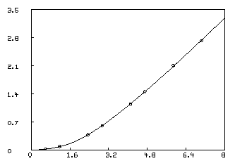
In order to visually see how our model with its parameters set to their best-estimated values corresponds to the data, we may draw a graph of the data points and the model function. Although we are drawing only the simplest and most direct kind of picture here, it should be noted that MLAB provides facilities for many types of point-symbols and types of lines, axes with arbitrarily-placed numeric labels in various formats, titles in the form of text strings in arbitrary sizes and various fonts with subscripts and superscripts, color, and a number of other special features. It is quite possible to prepare more or less elaborate publication-quality graphs with a modest amount of effort. Indeed this is one of MLAB's most-used facilities. The desired graph can be constructed as follows.
* draw D, linetype none,pointtype circle
* draw c2 = points(F,0:8:.2)
* VIEW

The first DRAW command above plots the data points, while the second
draw command constructs a curve called C2, which is a graph consisting
of solid straight-lines connecting the points which are the rows of
the 2-column matrix which is the value of the expression
POINTS(F,0:8:.2). This matrix has the values 0 through 8 in steps of
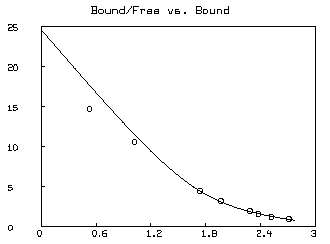
Often a Scatchard graph of Bound/Free vs. Bound (i.e.,
* SAVE W IN GW
* DELETE W
* FUNCTION R(X,Y)=IF Y=0 THEN (k1*s10+k2*s20) ELSE X/Y
* MF = F ON 0:8:.2
* M = B ON MF
* M = M&'(R ON M&'MF)
* DRAW M;
* MF = D COL 2
* M = (D COL 1)-(1+C)*MF
* M = M&'(R ON M&'MF)
* DRAW M, LINETYPE NONE, POINTTYPE "o"
* TOP TITLE "Bound/Free vs. Bound"
* VIEW
* DELETE W,MF,M
* USE GW
The &' operator denotes column concatenation, while the ON operator, as in F ON H, applies the function F to each row of the matrix H treated as an argument list for F and returns the column vector of result values.
It is an enlightening exercise to fit the Scatchard model to the
corresponding transformed data and to then draw a graph of the
original data points and the function
If we know we have non-cooperative two-site specific binding, with our
given
The non-specific binding constant,
If we have no such independent estimate of
* tolsos = .0002
* c = 0
* fit(k1,k2), F to d, constraints q
final parameter values
value           error           dependency      parameter
10.42883512     881.9654883     0.9989885554    K1
10.87461407     712.3997932     0.9989885554    K2
27 iterations
CONVERGED
best sum of squares = 1.31885e+00
root mean square error = 4.68838e-01
deviation fraction = 2.57765e-01
R squared = 8.02989e-01
no active constraints
LSQRPT is a sum of zero or more of the values 1, 2, 4, and 8. When LSQRPT contains 1, the best sum of squares obtained at each iteration is typed-out. When LSQRPT
We may examine our fit by redefining the curve C2.
* draw c2 = points(F,0:8:.2); view
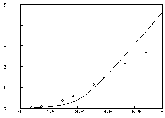
This is not an adequate fit, as we could have predicted by noting the large parameter standard deviations and the large RMS error. Although the dependency values are not extremely close to one, we may consider the possibility that our fit is bad because we fell into an unfortunate local minimum. A crude way to study this possibility is to draw a contour map of the sum-of-squares surface to see if several local minima are apparent. This is possible in this case, since we have fewer than three parameters, and MLAB can be used to view the sum-of-squares surface as follows. Drawing this contour map is time-consuming due to the large number of root calculations required.
* FUNCTION FH(F0,K1,K2)=ROOT(Z,0,F0,F0-(K1*S10*Z/(1+K1*Z)
       +K2*S20*Z/(1+K2*Z))-Z*(1+C))
* FUNCTION S(k1,k2)=SUM(I,1,8,(FH(D[I,1],k1,k2)-D[I,2])2)
* M=contour(points(S,cross(0:20,0:20)),1.3:1.35:.005&1.4:1.8:.2&2:5)
* DELETE W
* DRAW M, LINETYPE VMARKER; VIEW
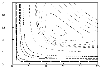
The CROSS operator expression above constructs a 441 by 2 matrix whose
rows are all the pairs
We may try a one-site model with
* S10 = S10+S20; k2 = 0;
* fit(k1,c), F to d, CONSTRAINTS Q
final parameter values
value           error           dependency      parameter
2.325176617     0.2567377717    0.5948957102    K1
0.4642651058    0.03442515131   0.5948957102    C
15 iterations
CONVERGED
best sum of squares = 1.55348e-02
root mean square error = 5.08835e-02
deviation fraction = 2.31134e-02
R squared = 9.97679e-01
no active constraints

*delete w
*draw D, line none, pointtype circle
*draw points(f,0:8:.2); VIEW
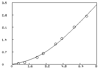
This fit is not as good as the fit obtained with the two-site model, and we can probably reject it. We should have an estimate of the variance of the data in order to test the goodness-of-fit. Even with curve-fitting evidence, it is best if there is independent evidence of multiple sites. Also, of course, a three or more site model, with or without non-specific binding may be the correct model.
Thus, in general, given the correct model, curve-fitting is a powerful device for estimating parameters; but curve-fitting is not always a very good way to distinguish the correct model from alternate impostor models. Usually we must resort to discriminating experiments.
MLAB can handle simultaneous curve-fitting, where several functions
are to be fit to corresponding sets of data points and where,
moreover, these several functions share some parameters in common.
MLAB model functions can be functions of more than one formal
argument, so that data points may lie in
Suppose we not only have the data given above for 2-site binding, but
also are given the following observations of the concentrations
   F0	   Y
  1.1734   .3
  2.5      .5
  3        .3
  3.98     .7
  6.5     1.6
Then we may enter this data as the rows of a matrix
* N=KREAD(5,2)
1.1734	.3
2.5	.5
3	.3
3.98	.7
6.5	1.6
In general, we should use weights which specify the relative accuracy
of each data point. For each data matrix, a vector of weight values
may be given as a clause in the FIT statement. The weight-value,
The use of weights permits data points of high reliability to exert greater influence on the parameter estimates than data points of lesser reliability. When simultaneous fitting is being done, weights have the additional function of compensating for differing units or magnitudes of the observations from various data sets. Without weights, the curve-fitting process would tend to favor one model component, fitting it at the expense of others, if the deviations there were much larger than the others, even though this may be an artifact of the use of different units.
MLAB includes an operator, EWT, which computes a vector of weight-values for a given set of data points, M, by estimating the standard deviation at each point by the difference between the data curve and a smoothed form of it, which effectively assumes the error is due to white noise. These standard-deviation estimates are, in turn, smoothed, and then used to form reciprocal variance weight values. In our example, we shall use EWT to obtain the necessary weight vectors, although this is not totally appropriate for chemical binding data, which is often taken in a range where the measurement accuracy improves as the amount of bound ligand increases. Also, EWT is unreliable for small numbers of data points. Nevertheless, we shall proceed as follows.
* DW = EWT(D); DN = EWT(N)
* TYPE D&'DW,N&'DN

: a  8 by 3 matrix
1:  0.58668    0.036    340.092919
2:  1.1734     0.096    340.092919
3:  2.3467     0.385    271.140209
4:  2.9334     0.61     256.511957
5:  4.1068     1.15     193.017413
6:  4.6934     1.46     171.441311
7:  5.8668     2.11     93.14747
8:  7.0402     2.73     93.14747

 a  5 by 3 matrix
1:  1.1734     0.3      159.445918
2:  2.5        0.5      159.445918
3:  3          0.3      156.341715
4:  3.98       0.7      134.665471
5:  6.5        1.6      134.665471

* fit (k1,k2,c), F to d with weight dw, Y to n with weight dn, CONSTRAINTS q
Begin iteration 1 bestsosq=5.86711e+01
Begin iteration 2 bestsosq=2.76531e+01
Begin iteration 3 bestsosq=2.69881e+01
final parameter values
value           error           dependency      parameter
1.681292363     0.3984166729    0.6190759098    K1
1.905413519e-17 0.06987097833   0.6367292361    K2
0.6401358429    0.057666687     0.09280130233   C
3 iterations
CONVERGED
best sum of squares = 2.69879e+01
root mean square error = 1.64280e+00
deviation fraction = 6.88260e-02
lagrange multiplier[1] = -0
lagrange multiplier[2] = -73.23991748
lagrange multiplier[3] = -0
* delete w
* draw d line none pt circle
* draw points(F,0:8:.2)
* draw n line NONE pointtype "+"
* draw points(Y,0:8:.2) linetype dashed
* VIEW

As mentioned above MLAB also allows weights to be the reciprocals or other functions of
the actual squared deviations themselves. This device is called
curve-fitting with iterative reweighting and is invoked in MLAB by
specifying an appropriate weight function. Moreover MLAB employs an
iterative reweighting technique to allow the general form of a sum of
pth powers to be minimized, rather than just a sum-of-squares. This
so-called
Given a radioactively-labeled ("hot") ligand material F, we wish to mix varying amounts of hot ligand each with the same fixed amount of site material, and obtain a table of the amounts of bound ligand corresponding to the total amounts of ligand added. This requires that we be able to separate the bound ligand from the free ligand and then measure the amount of bound ligand by the numbers of radioactive-decay events per minute for each distinct experiment.
There is an alternate device which sometimes has an advantage in simplicity over this direct method. Let us add a single fixed amount of hot ligand to the site material and then add varying amounts of unlabeled ("cold") ligand. The cold ligand form of F competes with the hot ligand in binding to the sites, and the effect is that as we add more cold ligand, the observed concentration of bound hot ligand decreases. We may sometimes be able to add an incremental amount of cold ligand to our mixture, separate and measure the amount of bound hot ligand, and then remix and add the next incremental amount of cold ligand; when this is possible, the variability due to differing concentrations of sites and hot ligand is reduced. Since replicate experiments suffer from using slightly-differing amounts of site material and of hot ligand, it is often better to expend effort getting more points for a single sample of site material than to run replicate experiments (except as a gross check on the experimental process.) In any event, the results of replicate experiments need not be averaged; the MLAB curve-fitting process will, in effect, give each point equal weight as is appropriate.
We have a further complication to deal with. Both the hot and cold
ligand materials usually bind weakly and non-specifically
throughout our
mixture, in addition to specifically binding with the site material. The
amount
In any event, for each observation point, we know the constant
Molar concentration
Then we have
The concentration of cold ligand is
Let us consider a single-site material
Our goal is to estimate
A pre-computer-style Scatchard-plot analysis method is often employed
to estimate the equilibrium constant
For a sequence of competitive binding experiments, the crucial point
is that when we have
When
In general, however, it is preferable to use the data (
Thus we may construct the data points (
A general do-file based on the MLAB statements given above can be
constructed which queries the user for the experimental parameters:
"liganal.do = competitive single site binding analysis"
echodo=0 /* echodo=0 inhibits screen and log-file output */
reset
namesw=0

type "Specify the COLD ligand molecular weight"
wc=kread("wc=")

type "Specify the HOT ligand molecular weight"
wh=kread("wh=")

type "Specify the half-life in days of the HOT ligand label"
hl=kread("hl=")

type "Specify the age in days of the HOT ligand label"
al=kread("al=")

type "Specify the counting-efficiency (c+/-/d+/-) of the label"
ce=kread("ce=")

type "Specify the counting time-period in minutes"
ct=kread("ct=")

type "Specify the background radioactivity in cpp(counts per period)"
br=kread("br=")

type "Specify the specific activity of the HOT ligand(in d+/-/mole)"
sa=kread("sa=")

type "Specify the total counts per period of HOT ligand(in cpp)"
tc=kread("tc=")

type "Specify the HOT ligand bindability fraction"
bd=kread("bd=")

type "Specify the Volume (in milliliters)"
v=kread("v=")

type "Specify the mass in ng of the HOT ligand
 (or enter -1 to have the mass computed for you.)"
mh=kread("mh=")

/*Compute the mass in ng of the HOT ligand! */
mhx=(v*wh*1e6)*(1e3/sa)*(tc/(ct*ce))*(2(al/hl))/v
type "specified mh value (in ng):", mh
mh=mhx
type "computed mh (hot mass) value (in ng) based on tc:",mh

type "Specify the number of experimental observation points"
nb=kread("nb=")
type "type-in the sequence of "+strval(nb)+" data points"
type  "as: ([COLD ligand mass in ng], [observed bound cpp]) pairs"
type  "on successive lines"
namesw=1
d=kread(nb,2); d=sort(d)

/* 2 classes-of-sites binding model.
   We use k2=0 and s20=0 for the 1-class-of-sites specialization*/
FCT A(F0)=G(F(F0))
FCT G(F)=B(F)+C*F
FCT B0(F0)=B(F(F0));
FCT B(F)=K1*S10*F/(1+K1*F)+K2*S20*F/(1+K2*F);
FCT F(F0)=ROOT(Z,0,F0,F0-B(Z)-Z*(1+C));
FCT Y(F0)=C*F(F0);
CONSTRAINTS CQ={K1>=0,K2>=0,C>=0,S10>=0,S20>=0};

lh=mh/(wh*v*1e6)
lhck=(tc/(ct*ce))*(1e3/sa)*(2^(al/hl))/v
namesw=0
type "Molar conc. of HOT ligand based on supplied molecular wt.",lh
type "Molar conc. of HOT ligand based on total cpp supplied",lhck
namesw=1

lh=lh*bd /* compensate for inert hot ligand */

fct m0(x)=if x>0 then x else 0
fct cconc(mc)=mc/(wc*v*1e6)
fct bconc(a0)=((a0-br)/(ct*ce))*(1e3/sa)*(2^(al/hl))/v

dm col 1 = cconc on (d col 1)  /*total cold (M)*/
dm col 2= m0 on bconc on (d col 2)   /*bound + non-spec. bound (M)*/

/*type-out the raw and converted input data*/
type "D=input data [Cold Ligand (ng) | Hot counts]", d
type "DM=[Cold Ligand (M) | Hot Spec.+Non-Spec.bound(M)]",dm

/* compute da col 1= LH+LC, da col 2= AH/alpha */
da=lh+(dm col 1)            /*total (hot+cold) */
alpha=lh/'da                /* vector of scale-factors*/
da col 2=(dm col 2)/'alpha  /* scaled bound+non-spec. bound */

/* compute guesses for K1 and S10 from the Scatchard fit.
   estimate C from the largest cold ligand data point. */

i=maxrow(dm col 1);
c=m0(dm[i,2]/(lh-dm[i,2]))

fre=lh-(dm col 2)            /*free hot (FH) in Molar units */
yns=c*fre                    /*non-spec. bound hot */
sd =m0 on ((Dm COL 2)-yns);  /* spec. bound hot*/
sd2 = sd/'fre                /*bound/free */
sd col 2=sd2
sd col 1 = (sd col 1)/'alpha /* spec. bound (all =H+C) */
sd=compress(sd);

type "directly-estimated non-spec. binding coef.", c

ltot=(da col 1)
ftot=((da col 1)-(da col 2))
ytot=yns/'alpha
btot = sd col 1

mmt=ltot&'btot&'ytot&'ftot
type "MMT=[L Total | B Total | Y Total | F Total]", mmt
mmh=mmt/'(alpha^^'4)
type "MMH=[L Hot | B Hot | Y Hot | F Hot]", mmh
mmcOA=mmt-mmh
type "MMC=[L Cold | B Cold | Y Cold | F Cold]", mmt

/*Remember BH/FH = -K1*BH/alpha +K1*S10 */

fct lin0(b)=-k1*b+k1s10 /* simple linear form */
fct lin(b) = -k1*(b-s10)
k1=1; k1s10=lh

lsqrpt=0
fit(k1,k1s10), lin0 to sd
s10=k1s10/k1
fit(k1,s10),lin to sd
type "Scatchard model linear-regession fit estimates",k1,s10
ok1=k1; os10=s10

draw sd lt none pt circle color orange
draw points(lin,0:s10!4) lt dashed
top title "Scatchard plot"
title "[dashed=regression-fit line]" at (.5,.75) fract size .14 inches
title "[hashed=euclidean-fit line]" at (.5,.7) fract size .14 inches

/* compute k1 and s10 for the best euclidean-fitting line */
qb=mean(sd)
q=sd-(qb')^^nrows(sd)
m=q'*q
z=eigen(m) row (1,3,5)
rno=if z[1,1]>z[1,2] then 2 else 3
v1=(z row rno)'
k1=-v1[2]/v1[1]
s10=(qb[2]-v1[2]*qb[1]/v1[1])/k1
type "Scatchard model euclidean-fit estimates;", k1,s10
draw points(lin,0:s10!50) pt nbar ptsize .01
unview;
ws=w; blank ws;

k2=0; s20=0;
/*define our weighting function (fixed-percentage error assumed) */
fct wvf(x)=1/x^p>
p=2;
wv1=.00000001*(wvf on (da col 2));

lsqrpt=8
maxiter=90
FIT(K1,s10,C),A TO da with wt (wv1), CONSTRAINTS CQ;

/* Draw the (full) relative saturation curve log-plot form ------------*/
FL = (da[1,1]*.9):((da[nrows(da),1])*1.1)!100;
am= POINTS(a,FL);
lda= (log on da col 1)&'((da col 2)/'(da col 1))
draw lda lt none pt circle ptsize .01
lam =(log on am col 1)&' ((am col 2)/'(am col 1))
draw lam

nk1=k1; ns10=s10; k1=ok1; s10=os10
am = points(a,fl)
k1=nk1; s10=ns10
lam =(log on am col 1)&' ((am col 2)/'(am col 1))
draw lam lt dashed
top title "Log-Percent Saturation Plot"
bottom title "log(TOTAL LIGAND)"
left title "(spec. bound)/(total)"
title "[dashed=regression-fit line]" at (.5,.8) fract size .15 inches
title "[solid=MLAB model-fit line]" at (.5,.75) fract size .15 inches
VIEW;

/*Now draw the Scatchard form of the data +fit-curves -------*/
w = ws; unblank w
draw points(lin,0:s10!4) color yellow
TOP TITLE "Scatchard Plot: Bound/Free vs. Bound" color green;
title "[solid=MLAB model-fit line]" at (.5,.8) fract size .14 inches
left title "(bound)/(free)"
bottom title "bound ligand"
lowy=minv(sd col 2); hiy=maxv(sd col 2)
window 0 to 2*s10, lowy to hiy adjust wnice
VIEW;
The MLAB log-file result of running the above do-file on some actual experimental data is shown below.
   MLAB Mathematical Modeling System, Revision: April 24, 1996
   Copyright: Civilized Software, Inc. (301)962-3711, email: csi@civilized.com

Sat May 18 15:29:38 1996
'* ' is the command prompt

* do liganal

Specify the COLD ligand molecular weight
wc=  1100
Specify the HOT ligand molecular weight
wh=  1130
Specify the half-life in days of the HOT ligand label
hl=  2
Specify the age in days of the HOT ligand label
al=  0
Specify the counting-efficiency (cpm/dpm) of the label
ce=  .5
Specify the counting time-period in minutes
ct=  5
Specify the background radioactivity in cpp(counts per period)
br=  0
Specify the specific activity of the HOT ligand(in dpm/mole)
sa=  2.5086e18
Specify the total counts per period of HOT ligand(in cpp)
tc=  65789
Specify the HOT ligand bindability fraction
bd=  1
Specify the Volume (in milliliters)
v=  .5
Specify the mass in ng of the HOT ligand
(or enter -1 to have the mass computed for you.)
mh=  -1
     specified mh value (in ng):
-1
     computed mh (hot mass) value (in ng) based on tc:
1.18538739E-2

Specify the number of experimental observation points
nb=  10
     type-in the sequence of 10 data points
     as: ([COLD ligand mass in ng], [observed bound cpp]) pairs
     on successive lines
  Type in numbers for KREAD.  End lines with ENTER
  0     8118
  .05   7694
  .1    7480
  .2    7080
  .5    6360
  1     6170
  3     5397
  10    5096
  30    5096
  1000  4714

     Molar conc. of HOT ligand based on supplied molecular wt.
2.09803077E-11
     Molar conc. of HOT ligand based on total cpp supplied
2.09803077E-11

     D=input data [Cold Ligand (ng) | Hot counts]

   D: a  10 by 2 matrix

  1: 0      8118
  2: 0.05   7694
  3: 0.1    7480
  4: 0.2    7080
  5: 0.5    6360
  6: 1      6170
  7: 3      5397
  8: 10     5096
  9: 30     5096
 10: 1000   4714

     DM=[Cold Ligand (M) | Hot Spec.+Non-Spec.bound(M)]

   DM: a  10 by 2 matrix

  1: 0                2.58885434E-12
  2: 9.09090909E-11   2.45363948E-12
  3: 1.81818182E-10   2.38539424E-12
  4: 3.63636364E-10   2.25783305E-12
  5: 9.09090909E-10   2.02822291E-12
  6: 1.81818182E-9    1.96763135E-12
  7: 5.45454545E-9    1.72111935E-12
  8: 1.81818182E-8    1.62512955E-12
  9: 5.45454545E-8    1.62512955E-12
 10: 1.81818182E-6    1.50330862E-12

     directly-estimated non-spec. binding coef.
  C = 7.71837904E-2

     MMT=[L Total | B Total | Y Total | F Total]

   MMT: a  10 by 4 matrix

  1: 2.09803077E-11   1.16933226E-12   1.41952208E-12   1.83914534E-11
  2: 1.11889399E-10   5.45935993E-12   7.62606519E-12   9.88039735E-11
  3: 2.0279849E-10    9.18445554E-12   1.38730875E-11   1.79740946E-10
  4: 3.84616671E-10   1.48997633E-11   2.64914424E-11   3.43225466E-10
  5: 9.30071217E-10   2.50658571E-11   6.48466349E-11   8.40158725E-10
  6: 1.83916213E-9    4.38447819E-11   1.28640441E-10   1.6666769E-9
  7: 5.47552576E-9    6.12326499E-11   3.87952055E-10   5.02634106E-9
  8: 1.82027985E-8    1.13851314E-10   1.29613305E-9    1.67928141E-8
  9: 5.45664349E-8    3.41291496E-10   3.88541133E-9    5.0339732E-8
 10: 1.8182028E-6     1.16933226E-12   1.30280259E-7    1.68792254E-6

     MMH=[L Hot | B Hot | Y Hot | F Hot]

   MMH: a  10 by 4 matrix

  1: 2.09803077E-11   1.16933226E-12   1.41952208E-12   1.83914534E-11
  2: 5.96713722E-10   2.91151354E-11   4.06703209E-11   5.26928266E-10
  3: 1.9602776E-9     8.87781883E-11   1.34099139E-10   1.73740028E-9
  4: 7.05089676E-9    2.73146488E-10   4.85648281E-10   6.29210199E-9
  5: 4.12306854E-8    1.11118638E-9    2.87469514E-9    3.72448039E-8
  6: 1.61223437E-7    3.84349283E-9    1.12767949E-8    1.46103149E-7
  7: 1.42902491E-6    1.59807452E-8    1.012493E-7      1.31179486E-6
  8: 1.57929939E-5    9.87789387E-8    1.12454254E-6    1.45696724E-5
  9: 1.41918596E-4    8.87644758E-7    1.01053353E-5    1.30925616E-4
 10: 0.15756973       1.01337083E-7    1.12903936E-2    .146279336

     MMC=[L Cold | B Cold | Y Cold | F Cold]

   MMT: a  10 by 4 matrix

  1: 2.09803077E-11   1.16933226E-12   1.41952208E-12   1.83914534E-11
  2: 1.11889399E-10   5.45935993E-12   7.62606519E-12   9.88039735E-11
  3: 2.0279849E-10    9.18445554E-12   1.38730875E-11   1.79740946E-10
  4: 3.84616671E-10   1.48997633E-11   2.64914424E-11   3.43225466E-10
  5: 9.30071217E-10   2.50658571E-11   6.48466349E-11   8.40158725E-10
  6: 1.83916213E-9    4.38447819E-11   1.28640441E-10   1.6666769E-9
  7: 5.47552576E-9    6.12326499E-11   3.87952055E-10   5.02634106E-9
  8: 1.82027985E-8    1.13851314E-10   1.29613305E-9    1.67928141E-8
  9: 5.45664349E-8    3.41291496E-10   3.88541133E-9    5.0339732E-8
 10: 1.8182028E-6     1.16933226E-12   1.30280259E-7    1.68792254E-6

     Scatchard model linear-regession fit estimates
  K1 = 138222119
  S10 = 3.0576542E-10

     Scatchard model euclidean-fit estimates;
  K1 = 287268836
  S10 = 1.82633621E-10

final parameter values
      value               error                dependency    parameter
   1187347821          228157865.8            0.9547016996     K1
   4.947046514e-11     8.636211996e-12        0.9633732247     S10
   0.0804516126        0.001324755233         0.5724726409     C
19 iterations
CONVERGED
best weighted sum of squares = 4.378871e-11
weighted root mean square error = 2.501106e-06
weighted deviation fraction = 1.716122e-02
R squared = 9.982448e-01
no active constraints
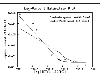
Note that the log-percent saturation plot using the estimated values
for K1 and S10 obtained by linear-regression
with the bound/free vs. bound Scatchard-plot form of the
data is decidedly inferior to the graph using the direct saturation
model-based estimates. Of course, as the following picture shows,
this situation is not so clear in the Scatchard plot
itself. But the log-percent saturation plot is the more faithful
form of the data with regard to minimal error in the
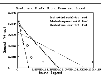
You can see that MLAB is an extremely flexible and general tool for curve-fitting. Moreover, it has a broad range of other useful functions, only a few of which have been alluded to here.